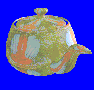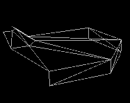
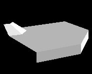
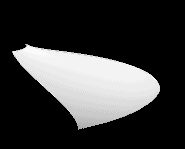
 Bezier control points as A) wireframe, B) shaded polygons, C) Generated patch
by Chris Bentley
Sixteen control points define an entire curved surface. Clearly one of the advantages of Bezier patches is that they allow a much more concise representation than vertex, polygon lists. Other virtues of parametric surfaces are that they provide exact analytical descriptions of surfaces, and permit easy deformations of those surfaces. Finally, if texture mapping is being performed, parametric surfaces are convenient because the (u,v) parameters used to generate the surface can easily be reused as (u,v) texture parameters.
There are, however, some disadvantages to using Bezier patches. In the first place, to render a parametrically defined patch, it is usually necessary to generate a vertex, polygon description of the object, and then render this. Also, given a set of 3D vertices, it may be hard to extrapolate out to the control points for this surface. Furthermore, if multiple patches are combined to form a description of a complex shape, there may be problems with normal interpolation across patch boundaries, and with cracks forming at patch boundaries


 Bezier control points as A) wireframe, B) shaded polygons, C) Generated patch
I. Bezier Formulation
There are several different ways of interpolating the control points of a 2D Bezier curve. Though different, these methods all generate the same points on the parametric curve. The first method, developed by P. Bezier, calculates points on the curve through weighted interpolation of the four control points.
Control points for Bezier curve:
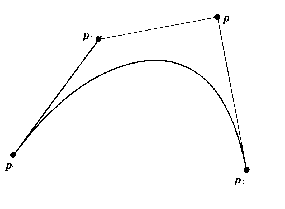
What contribution each control point makes to the curve depends on a single parameter, u, with 0 <= u <= 1. As u varies along the curve each control point's contribution varies as a function of u. In fact, each control point has a function which controls its influence; these are known as the Bernstein basis functions. If we look at the graph below, we see that the function for the first control point has a value of 1 when u = 0, and decays to 0 as u approaches 1. This means that the first control point contributes 100% to the curve when the curve is very close to it, and that when the curve is far away, it hardly contributes anything. The Bernstein basis functions cause Bezier curves to pass through the starting and ending control points.
Bernstein basis functions for Bezier curve:
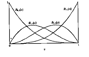
For a given value of u, a point Q on a Bezier curve is defined as the sum of the four control points, weighted by the value of the basis functions for that value of u:

And the Bernstein basis functions are defined as follows:


II. Midpoint Method
The points in a parametric Bezier curve can also be calculated by recursively halving the distance between neighboring control points. This method divides the original four control points into two smaller sets of Bezier control points, defining a "left" and a "right" Bezier curve. The last control point in the left curve coincides with the first control point in the right curve. Since, as stated earlier, Bezier curves pass through the first and last control points, this means this shared point is actually on the final parametric curve.
Applying this process recursively generates more points that are on the final curve, and this can be taken to any desired level of resolution. One particularly nice feature of this method is that it relies entirely on halving. Thus, if coordinate values are stored as fixed-point fractions, this method can be implemented exclusively using adds and "shifts", which are much faster than actual fractional divisions.
Points on Bezier curve by recursive subdivision:

In the above diagram:


III. De Casteljau Representation
The third method, developed by P. de Casteljau, is a generalization of Midpoint Algorithm. It turns out that halving the distance between control points is not the only way to calculate points on the curve. In fact, splitting the distance between neighboring control points in any ratio works just as well.
Points on Bezier curve by recursive subdivision, u = 0.6:

Applying the linear interpolation recursively, again, generates points on the curve to any level of resolution. In de Casteljau's formulation, the control points at any level of recursion are a linear combination of the neighboring control points from one level "higher":


where:


Turning now to 3D Bezier surface patches; these are defined by grid of
16 control points (4 rows, 4 columns). Each row of four control points
can be thought of as a separate 2D Bezier curve. If we first compute
a point on each of the curves for a given value of u , say 0.2,
we can then treat these new points as the control points for 2D Bezier
curves running down the columns. In this way points are interpolated
bilinearly to generate the surface patch. The Bezier curves which form
the boundaries of the patch will also be points in the 3D surface.
Thus, for a given value of (u,v), a point Q on a Cubic Bezier
surface can be defined as the weighted sum of all of the control points
in the patch:

 :
:


Implementaton of Mesh Generation
When rendering multiple patches, it is efficient to precalculate values for the Bernstein basis functions for fixed intervals of u and v, since every patch uses the same values for these functions. Here is the algorithm used to generate polygon mesh from Bezier patch:
A. Precalculate values for Bernstein basis functions:
        uinc = 1.0/steps;
        u = uinc;

        for( i = 1; i < steps; i++, u += uinc )
        {
                u_sqr = SQR(u);                 /* u^2 */
                tmp = 1.0 - u;                  /* (1-u) */
                tmp_sqr = SQR(tmp);             /* (1-u)^2 */

                B[0][i] = tmp * tmp_sqr;        /* (1-u)^3 */
                B[1][i] = 3 * u * tmp_sqr;      /* 3u(1-u)^2 */
                B[2][i] = 3 * u_sqr * tmp;      /* 3u^2(1-u) */
                B[3][i] = u * u_sqr;            /* u^3 */
        }
B. Use blending tables to calculate points in "row curve":
for( u = 0; u < 10; u++ )
{
    blend row 0 control points -> new control point
    blend row 1 control points -> new control point
    blend row 2 control points -> new control point
    blend row 3 control points -> new control point

    for( v = 0; v < 10; v++ )
    {
        blend 4 new control points -> point on surface
    }
}
C. Generate edges and polygons from grid of surface points.
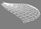
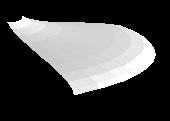
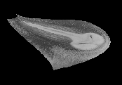 Bezier surface as A) triangle mesh, B) shaded triangles, C) texture mapped
This method has several advantages over the polygon mesh method. One major benefit is that subdivision generates a smooth silhouette in addition to smooth surfaces. This is something that is hard to achieve with polygon based rendering. Also, subdivision takes more compact data, since only control points need to be stored. Most importantly, since there are no polygons, there is no need for complex polygon scan conversion code; and since the subdivision algorithm is recursive it is very compact to code. Finally, subdivision takes care of problems with normals at patch boundaries.
The subdivision method also suffers from several disadvantages. The primary problem with the algorithm is that it is slow, because it requires subdivision both in world and screen space, and > 4 perspective calculations are needed for every pixel plotted. Another problem is that the maximum recursion depth depends on the screen coverage of the largest patch, and this seems like a vulnerability.
Implementation of Subdivision Rendering
1.     For each surface patch
1.1       project corner control points to screen space
1.2       if points project to one pixel
1.2.1           color that pixel
1.3       else
1.3.1           break patch into 2 subpatches
1.3.2           apply algorithm recursively to 2 subpatches
Implementation of Subdividing Patches
For example, row 0 of a grid of control points consists of control points:
P00, P01, P02, P03
Subdividing this will generate row 0 of left and right subpatches :
        Left.P00  = P00
        Right.P03 = P03

        Left.P01 = (P00 + P01)/2
        Right.P02 = (P02 + P03)/2

        tmp = (P01 + P02)/2

        Left.P02 = (Left.P01 + tmp)/2
        Right.P01 = (Right.P02 + tmp)/2

        Left.P03 = (Left.P02 + Right.P01)/2
        Right.P00 = Left.P03
The subdivision algorithm is slow for a number of reasons. In the first place, when we subdivide a patch, we need to subdivide world coordinates and normals. Secondly, to test whether a patch projects to 1 pixel, we need to maintain screen coordinates for the control points at the corners of the patch. Finally, for a patch to project to 1 pixel we must project all 4 corners of the patch to that pixel, which means we will perform > 4 perspective calculations per pixel plotted!
We can cut down on the number of projections to screen coordinates that we perform by recognizing that we only need to transform 2 new points per patch, since each patch inherits 2 corner control points from its "parent" patch. Also, we can improve the performance by doing "back patch" culling: if a patch has all of its corner normals backfacing, skip it.
Bezier surface patches rendered by converting to polygon mesh:
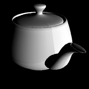
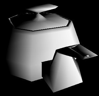
Bezier surface control points rendered as polygons:
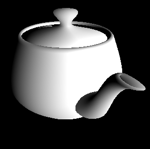
Bezier surface patches rendered by subdivision algorithm:
Cracking between Bezier patches subdivided to different depths:
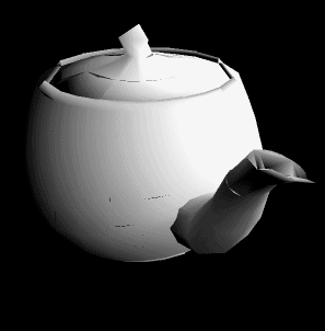
Bezier surface patches rendered with texture mapping:
