Curves are one of the most essential objects to create high-resolution graphics. While using many small polylines allows creating graphics that appear smooth at fixed resolutions, they do not preserve smoothness when scaled and also require a tremendous amount of storage for any high-resolution image. Curves can be stored much easier, can be scaled to any resolution without losing smoothness, and most importantly provide a much easier way to specify real-world objects.
All of the popular curves used in graphics are specified by parametric equations. Instead of specifying a function of the form y = f(x), the equations y = fy(u) and x = fx(u) are used. Using parametric equations allows curves that can double back and cross themselves, which are impossible to specify in a single equation in the y = f(x) case. Parametric equations are also easier to evaluate: changing u results in moving a fixed distance along the curve, while in the traditional equation form much work is needed to determine whether to step through x or y, and determining how large a step to take based on the slope.
The remainder of this document describes LeGrange interpolated curves, cubic B-splines, and Bezier curves. While LeGrange interpolated curves are not often used in computer graphics, they help give a simple foundation for understanding Bezier curves and B-splines, the most commonly used graphical curves.
The goal of LeGrange interpolation is to create a smooth curve that passes through an ordered group of points. When used in this fashion, these points are called the control points. The general idea, as with all curve algorithms, is to use the control points to generate parametric equations. To draw the curve, all that is then needed is to step through u at some small amount, drawing straight lines between the calculated points. The smaller the step size the more smooth the curve will appear. The step size can be calculated based on the amount of pixels available in the output image.
To do LeGrange interpolation, we wish to specify a curve that will pass through any number of control points. The curve's function can be constructed as a sum of terms, one for each control point.
  fx(u) = sum from i = 1 to n of x[i] B[i](u)
  fy(u) = sum from i = 1 to n of y[i] B[i](u)
Each function B[i](u) specifies how much the ith control point effects the position of the curve. This can be thought of as a function specifying how much the ith control point draws the curve towards it. The name for these functions are Blending Functions. If for some control point i the value of this function is 1 and for every other control point the value of this function is 0, the curve will go through i at that value.
To achieve the goal of LeGrange interpolation, getting a curve that passes through all the specified control points, the blending functions must be defined so that the curve will go through each control point in the proper order. This can be done by creating blending functions where the first control point is passed through (has total control) at u = -1, the second control point is passed through at u = 0, the third at u = 1, and so on. A mathematical expression that does so is:
u (u - 1) (u - 2) . . . [u - (n - 2)]
At u = -1 this expression is:
-1 (-2) (-3) . . . (1 - n)
So dividing the first by the second gives us 1 when u = -1, and gives us 0 when u is a whole number greater then -1 and less then or equal to n. Using this method for the other blending functions gives us the same type of behavior for the other control points. This function defines the LeGrange interpolation blending functions.
          (u + 1) (u) (u - 1) ... [u - (i - 3)] [u - (i - 1)] ... [u - (i - 2)]
B[i](u) = ---------------------------------------------------------------------
                  (i - 1) (i - 2) (i - 3) ... (1) (-1) ... (i - n)
To draw a curve using this, it is necessary to decide how many control points we will use for the basis of the curve, and then calculate the blending functions B[1](u) to B[n](u), where n is the number of control points. The final functions for x, y, and z are then:
  x = x[1] B[1](u) + x[2] B[2](u) + x[3] B[3](u) + . . . + x[n] B[n](u)
  y = y[1] B[1](u) + y[2] B[2](u) + y[3] B[3](u) + . . . + y[n] B[n](u)
Where x[i] is the x coordinate of the ith control point, and y[i] is the y coordinate of the ith control point.
The number of control points used is most commonly 4. In this case, the calculated curve is particularly good between the second and third control points (0 <= u <= 1). Thus to draw a full LeGrange interpolated curve using many control points, it is common to work with sets of four points. First start with the first through fourth control points, and step through u from 0 to 1 in small steps, drawing straight lines between each. When u = 1 is reached, switch to using the second through fifth control points. Now step through u from 0 to 1 in small steps again. Repeat this, each time shifting down along the control points in the curve by one point until the end of the curve is reached. At this point all of the curve will have been drawn, except for the first and last segments (the curve between the first and second control points and the curve between the second to last and last control points). These can be dealt with as special cases, calculating from -1 <= u <= 0 using the first four control points and 1 <= u <= 2 using the last four control points.
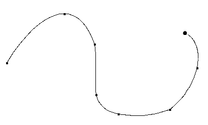
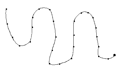
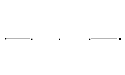
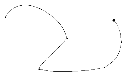
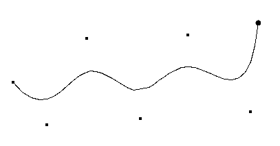
Some sample LeGrange interpolated curves appear below.


The last two of the above images shows why LeGrange interpolated curves are not usually used in graphics. Although the control points form a straight line, the curve wiggles between the control points. This results because the blending functions sum to 1 at the control points, but do not necessarily do so at fractional values. To eliminate the wiggle we would need to dividing the value of each blending function by the sum of the blending function values before using them. However, there is also another problem. While each section of the curve connects to the next section at a control point, the slopes for the connected curves at the control point may be different. This results in the ability to have corners at control points. This results because while at control points only that control point has control, at any other part of the curve all points have some control. The third problem is that the LeGrange curve goes outside the convex hull of the control points. This means that clipping LeGrange curves must be done with every single line segment drawn, instead of clipping the control points and then just drawing the curve. This adds much computation.
B-splines correct the deficiencies of LeGrange interpolated curves by defining blending functions that vary each control point's control from 0 far away from the point to its maximum near the point. This can be done by making it so the curve does not pass through each control point, but instead just passes near them. The sum of the B-Spline blending functions also always sum to 1, and the slopes between curve segments are continuous. Finally, the final curve always lies within the convex hull of the control points.
While B-splines can be of higher order, usually cubic B-splines are used. Cubic functions allow for enough curve flexibility for most tasks, and are easier to work with then higher order functions since they behave more predictably (higher order functions may get unexpected wiggles and kinks). The cubic B-Spline blending functions work over four control points. The blending functions appear below. Note that special blending functions are needed for the first and last two sections of the B-Spline so that it passes through the first and last points.
  First section:
  B[1](u) = (1 - u)^3
  B[2](u) = 21 u^3 / 12 - 9 u^2 / 2 + 3 u
  B[3](u) = -11 u^3 / 12 + 3 u^2 / 2
  B[4](u) = u^3 / 6

  Second section:
  B[1](u) = (1 - u)^3 / 4
  B[2](u) = 7 u^3 / 12 - 5 u^2 / 4 + u / 4 + 7 / 12
  B[3](u) = - u^3 / 2 + u^2 / 2 + u / 2 + 1 / 6
  B[4](u) = u^3 / 6

  Middle sections:
  B[1](u) = (1 - u)^3 / 6
  B[2](u) = u^3 / 2 - u^2 + 2 / 3
  B[3](u) = - u^3 / 2 + u^2 / 2 + u / 2 + 1 / 6
  B[4](u) = u^3 / 6

  Second to last section:
  B[i](u) = F[5 - i](1 - u) where F[i](u) is the ith blending function for
  the second section.

  Last section:
  B[i](u) = F[5 - i](1 - u) where F[i](u) is the ith blending function for
  the first section.
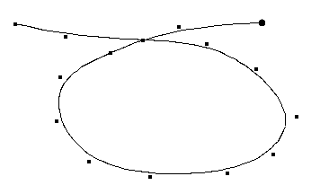
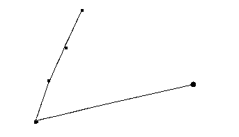
Note that B-Spines are designed to eliminate sharp corners, as seen above. A sharp corner can be obtained, however, by using duplicate sequential control points. Using three identical control points causes the curve to pass through the point, as illustrated below.
Bezier curves are another very popular curve type. Bezier curves, unlike B-splines, must have precisely n control points, where n + 1 is the degree of the Bezier polynomial. To create a longer curve, it is necessary to connect multiple Bezier curves. This is usually done by making the last control point of one curve the same as the first control point of the next curve. Bezier curves pass through the first and last control points of each curve segment, however, which makes them quite easy to work with and popular for use in interactive design programs. Bezier curves, like B-Spline curves, always lie within the convex hull of the control points, and always have the sum of the basis functions add to 1.
The idea behind Bezier curves is quite simple. To create a smooth curve, one intuitive mechanism is to first connect the four control points with lines. Then draw new lines connecting the midpoints of those lines, and more new lines to connect the midpoints of the new lines, and so forth until the resulting curve is sufficiently smooth. This is illustrated below.
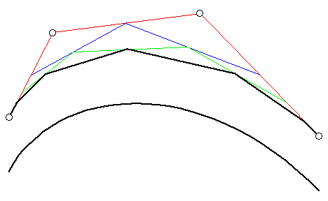
While it is possible to define a curve type based on connecting the last third of one segment to the first third of the next, or the last fourth of one segment to the first fourth of the next, and so on, using midpoints allows for a very efficient subdivision algorithm to be derived.
The basis functions for cubic Bezier curves, which have the same results as the above subdivision process, appear below. These are based on Bernstein polynomials.
  B[1](u) = (1 - u)^3
  B[2](u) = 3 u (1 - u)^2
  B[3](u) = 3 u^2 (1 - u)
  B[4](u) = u^3
The DeCasteljau representation of Bezier curves is usually used, however. This is a recursive definition of the above polynomials that is based on the subdivision illustrated earlier.
   r                 r-1         r-1
  p[i](u) = (1 - u) p[i](u) + u p[i + 1](u)

where
  p[1], p[2], . . ., p[n] are the control points
  r = 1, 2, . . ., n
  i = 0, 1, . . ., n - r
  p[i](u) = p[i]

A point on the curve is given by p[0]^n (u).
Using this derivation, it is possible to see a simple recursive subdivision process for generating cubic Bezier curves. This works by taking the original Bezier curve and breaking it into two smaller Bezier curves, as illustrated below. These Bezier curves can then be broken into smaller Bezier curves, and so on, until the control points of the Bezier curve are very close to a straight line. When this happens, a straight line is drawn between the first and last control points, and the recursion pops back up.
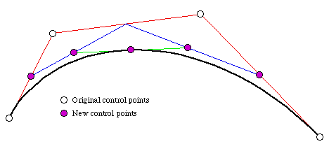
At each stage of subdivision, the control points of the sub-curves are calculated by:
  q[0] = p[0]
  q[1] = (p[0] + p[1]) / 2
  q[2] = (q[1] / 2) + (p[1] + p[2]) / 4
  q[3] = (q[2] + r[1]) / 2

  r[0] = q[3]
  r[1] = (p[1] + p[2]) / 4 + (r[2] / 2)
  r[2] = (p[2] + p[3]) / 2
  r[3] = p[3]
where p[1..4] are the control points of the original Bezier, and q[1..4] and r[1..4] are the control points of the sub-curves. This derivation was first done by Lane.
The linearity test for the above method is quite simple: all that needs to be done is calculate the sum of the distance from points p[1] and p[2] to the line connecting p[0] and p[4], and see if this is greater then some tolerance.
All of the above can be applied to 3-D curves by including a third equation to specify z:
fz(u) = sum from i = 1 to n of z[i] B[i](u)
and using the same blending functions. The optimized version of the Bezier curve formulation, however, would need to be changed.
The LeGrange interpolation and the cubic B-Spline information, including the blending functions, are from "Computer Graphics, A Programming Approach", written by Steve Harrington, 1987.
The Bezier information comes from "Advanced Animation and Rendering Techniques, Theory and Practice" by Alan Watt and Mark Watt, 1992.
meyerd@cs.WPI.EDU