 Images
by Chris Bentley
AVS (Advanced Visualization System), described by Craig Upson [UPSON89], is one of the dominant visualization packages available today. AVS provides "modules" which each perform some visualization technique, and a user interface which allows these modules to be connected together in the manner of a flow chart. Data that is input to the system, is processed by the modules in the sequence ("network"), and then usually an image is produced. AVS thus implements a data-flow paradigm of scientific visualization. The AVS interface provides a form of visual programming language, in which the user can manipulate icons for the modules to build a new "flow program".
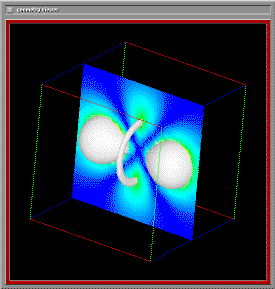
The image below shows both the raw data for field density values around a hydrogen atom, as well as the visualization of this data. The rendering encorporates several display techniques: isosurface rendering, and arbitrary slicing, to allow a user to develop a more intuitive grasp of the data.
Numeric Data  Images
000 000 000 001 000 000 000 000
000 000 000 000 000 000 000 000
000 000 000 001 002 003 005 007
011 013 016 021 023 026 031 033
034 036 036 036 036 034 033 031
026 023 021 016 013 011 007 005


Fig 1. Hydrogen atom data
Two dimensional data, such as readings taken from some surface, can of course be displayed as images. However, much of the data that AVS accepts is 3 dimensional in nature. Researchers working in computer graphics and visulaization have developed a large repetoire of methods for rendering 2D and 3D data. Among these methods are:
etc ...
Raw Numeric Data


Selected Numeric Data


Process Numeric Data


Geometric Data


Images
Modules
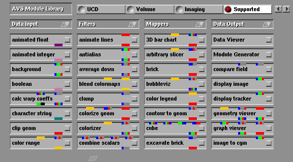
The image below shows the organization of AVS modules on the screen. There are four main columns corresponding to the four module types. The user can scroll up and down in each of the columns which are menus. Once a desired module has been located the user can click the mouse button on the module's icon and "drag" the module into a workspace area.

Fig 2. AVS module palette
Widgets
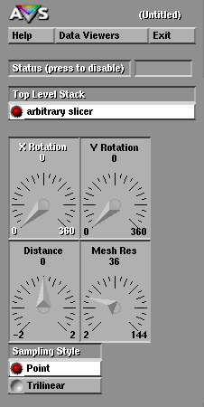
Once it is instantiated, each module can have control "widgets" associated with it, such as dials and sliders. Turning a dial or pressing a push-button will cause the module to recompute its data. Thus the widgets give the user control over the visualization process.

Fig 3. AVS widget controls
Networks
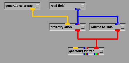
Modules have small, color coded "ports" on their upper and lower sides indicating what types of data they accept, and what types they output. By connecting "pipes" from the output port on one module to the input port on another, the user can specify the sequence of processing to perform on the data. Thus, AVS provides a user interface for linking modules into "networks". The network specifies how data flows between the modules. In the example shown below, in Fig. 4, the read field module reads data in from a file in disk. The generate colormap module outputs a table associating colors with certain numeric values. The field data flows from read field through the blue "pipes" to two modules: arbitrary slicer and volume bounds. The data is converted by these modules into geometric primitives which can be passed on to the geometry viewer module for final rendering.

Fig 4. AVS flow network
There are over 100 AVS modules already written; many visualization tasks can be performed by combining these modules into flow networks. The number of possible network permutations is huge. However, AVS can also be extended, by adding new modules written by the user or by third parties. AVS provides a C programming interface for writing modules. The structure of a module is very simple. It consists of 3 functions: an init function, a description function, and a compute function:
AVSinit_module()
{
        /* tell AVS name of description function */
}

static int description_function()
{
        /* set module name */

        /* setup input/output ports & any widgets */

        /* tell AVS name of compute function */
}

static int compute_function( input, output )
{
        /* operate on input and output */
}
#include < stdio.h >
#include < sys/types.h >
#include < sys/stat.h >
#include < fcntl.h >
#include < limits.h >

#define WIDTH   400
#define HEIGHT  400

unsigned int image[WIDTH][HEIGHT];

/**********************************************/
main()
{
        generate_image();
        write_image();
}

/**********************************************/
generate_image()
{
        int x, y;

        for( y = 0; y < HEIGHT; y++)
            for( x = 0; x < WIDTH; x++ )
                image[y][x] = (x+y)%256;
}

/**********************************************/
write_image()
{
        int             fd, y;
        unsigned int    width = WIDTH;

        if( (fd = open( "image.x", O_WRONLY|O_CREAT, 0777 )) < 0  )
        {
                fprintf( stderr, "Error opening file\n" );
                exit( 1 );
        }

        if( write( fd, (char*)&width, sizeof(unsigned int) ) < 0  )
                fprintf( stderr, "write error - width\n" );

       if( write( fd, (char*)&width, sizeof(unsigned int) ) < 0  )
                fprintf( stderr, "write error - height\n" );

        for( y = 0; y < HEIGHT; y++)
            if( write( fd, (char*)image[y], width*sizeof(unsigned int) ) < 0  )
                fprintf( stderr, "write error\n" );

        close( fd );
}