CS 2223 Mar 31 2023

Lecture Path: 11
Back Next

1 Open Addressing / Linear Probing

1.1 HW2 Ideas

If you want some ideas for How to maintain a linked list in ascending order, consider reviewing OrderedLinkedList).

1.2 Announcements on office hour updates

If a TA/SA cannot make a regularly scheduled office hour, then an announcement will be posted in Canvas with the adjusted datetime. Please double-check in canvas if you think an office hour is not being covered.

1.3 Sorting Summary

Another general shout!
I do believe that these applauses
are for some new honours
that are heap’d on Caesar.
Julius Caesar
William Shakespeare

We could have spent several weeks on sorting algorithms, but we still have miles to go before we sleep, so let’s quickly summarize. We covered the following:

• Insertion Sort

• Selection Sort

• Merge Sort

For each of these, you need to be able to explain the fundamental structure of the algorithm. Some work by dividing problems into subproblems that aim to be half the size of the original problem. Some work by greedily solving a specific subtask that reduces the size of the problem by one.

For each algorithm we worked out specific strategies for counting key operations (such as exchanges and comparisons) and developed formulas to count these operations in the worst case.

We showed how the problem of comparison-based sorting was asymptotically bounded by ~N log N comparisons, which means that no comparison-based sorting algorithm can beat this limit, though different implementations will still be able to differentiate their behavior through programming optimizations and shortcuts.

1.4 Homework2

Be sure to replace "USERID" with your CCC credentials. For example, my email address is "heineman@wpi.edu" so my USERID would be "heineman".

Pro tip: Don’t create a folder "USERID.hw2" – Make sure that on your file system there is a folder "USERID" and inside this folder is another folder "hw2".

1.5 Linear Probing

The linked list structure of SeparateChainingHashST seems excessive, although it does deliver impressive results. Is there a way to use the hash(key) method in a different manner? It will still return values between 0 and M-1, but what if we just created an array of M potential values, and tried to use the computed hash(key) to find an index location where we can put the value associated with that key?

In this situation, all we want to do is store the key to be able to determine later whether the key is in the array or not. What if we just used hc = hashcode(key) % M, where M is the array length, to determine the index position in which to place the key?

In in = new In ("words.english.txt"); String[] knownStrings = new String[1000003]; int numCollisions = 0; while (!in.isEmpty()) { String word = in.readString(); int location = (word.hashCode() & 0x7fffffff) % knownStrings.length; if (knownStrings[location] == null) { knownStrings[location] = word; } else { System.out.println("COLLISION between " + knownStrings[location] + " an " + word + " on " + location); numCollisions++; } System.out.println(numCollisions + " total collisions."); } in.close();

Run this code and see what happens. It takes every word from the dictionary of English words and tried to find a unique location where that word would be placed. There are 321,129 words, so let’s start with an array containing just over one million values. Is this enough?

When you run, you see there are 46,334 collisions, that is, a situation where two (or more) keys are mapped to the same index location using the modulo array length technique.

Can we fix this situation by making the array larger? With the aim to increase storage and thereby reduce the chance of a collision?

N # Collisions 1000003 46334 total collisions 2000006 24403 total collisions 4000012 12491 total collisions 8000024 6215 total collisions 16000048 3136 total collisions 32000096 1523 total collisions 64000192 747 total collisions 128000384 362 total collisions 256000768 183 total collisions 512001536 84 total collisions 1024003072 44 total collisions

As the size of the array doubles in size, the number of collisions appears to be cut in half. There is nothing magical here – just mathematics, so you can move along.

Still, this approach might be the basis of something useful. Again, let’s take a flawed approach and change things slightly to create an approach that always works, as long as the size of the storage array is greater in size than N, the number of keys being stored.

1.6 Open Addressing

Open addressing resolves hash collisions by probing (or searching) through alternative locations in an array when the modulo computation encounters a collision. One common approach, called linear probing, resolves collisions by checking for a higher index position in the array that is empty, into which the key is stored. If the end of the array is reached without finding an empty location, start over from index position 0. This search is guaranteed to succeed because there will always be an empty index location.

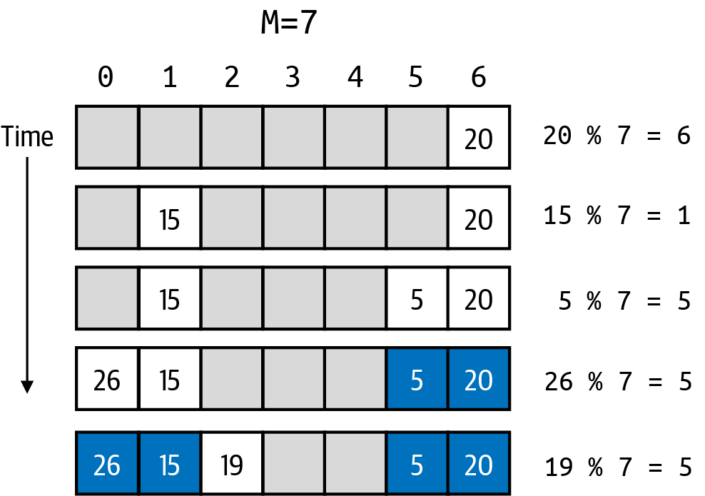
In this example, the first three keys (whose computed locations of 20, 15 and 5) all are inserted without any problems.

This sure looks great! But when the fourth key is inserted, its computed location of 5 is already occupied! Simply advance to the right (starting back over at index location if you run out) and find the first empty location and that is where you place the key.

Repeat once more with a key whose index location turns out to be 5 again. Now you can see that an increasing number of index locations have to be explored before finding an empty spot.

A chain of entries for a given index location in an open addressing Symbol Table is a sequence of consecutive non-null index locations in keys. This sequence starts at a given keys[hc] and extends to the right (wrapping around to the first index in table as needed), up to but not including the next available unused table index position. In the figure ealier, the chain for hc of 5 has a length of 5 even though there are only three entries whose key hashes to that same code. Also, there are no keys with a hash code of 2, but the chain for hash code 2 has a length of 1 because of an earlier collision. The maximum length of any chain is M–1 because one bucket is left empty.

You might wonder why this approach will even work. Since entries can be inserted into an index location different from hc = hash(key) % M, how will you find them later? The answer is that you search for a key in the exact same manner in which you put the keys into the array.

If we are going to use this approach to store (key, value) pairs, then we will need to create two "parallel" arrays of same length, where the corresponding index locations reflect that vals[i] is associated with keys[i].

The following is a simplifed implementation of a Symbol Table implemented using linear probing. For the structure, we need to keep track of two arrays of equal length.

public class LinearProbingHashST<Key, Value> { // Simplified from Book... int N; // number of key-value pairs in the symbol table int M; // size of linear probing table Key[] keys; // the keys Value[] vals; // the values public void put(Key key, Value val) { int i = hash(key); while (keys[i] != null) { if (keys[i].equals(key)) { vals[i] = val; return; } i = (i + 1) % M; } keys[i] = key; vals[i] = val; // (key, val) is now associated in ST. N++; } }

Then we find the initial location where a key is hashed. From that location, we search until keys[i] == null since that is where the key should be placed. Note that we also increase N to remember how many (key, value) pairs are in the Symbol Table.

To determine whether there is a corresponding value for a key, we repeat the process: starting at the index location determined by hash(key), search until you have either found the key you are looking for – in which case simply return the associated value – or search until you reach an index location containing the null value, which signifies that the key does not exist in the symbol table.

public Value get(Key key) { int i = hash(key); while (keys[i] != null) { if (keys[i].equals(key)) { return vals[i]; } i = (i + 1) % M; } return null; }

1.7 Resizing

Using the same technique of geometric resizing, the size of the storage array will continuously grow to ensure that there will be sufficient empty index locations. Once more than half of the index location in keys[] are occupied, both arrays are doubled in size, as you have seen me do on a number of occasions.

void resize(int capacity) { LinearProbingHashST<Key, Value> temp = new LinearProbingHashST<Key, Value>(capacity); for (int i = 0; i < M; i++) { if (keys[i] != null) { temp.put(keys[i], vals[i]); } } keys = temp.keys; vals = temp.vals; M = temp.M; }

As was done with the linked list implementation, a new LinearProbingHashST object is constructed with the desired extra capacity, and each (key, value) pair that exists in the original array will be put into the temporary LinearProbingHashST object. Then the original object just steals the two arrays (keys and vals) and increases M to reflect the new array lengths.

1.8 Removing a key from LinearProbingHashST

Removing a (key, value) pair from open addressing is going to be tricky. Let’s go back to the figure earlier.

What if you wanted to remove the key whose hash code was 20, and which appeared in index location 6? Perhaps you can remove it by setting the key at that location to null. Doing this would break the chain that starts at index location 5.

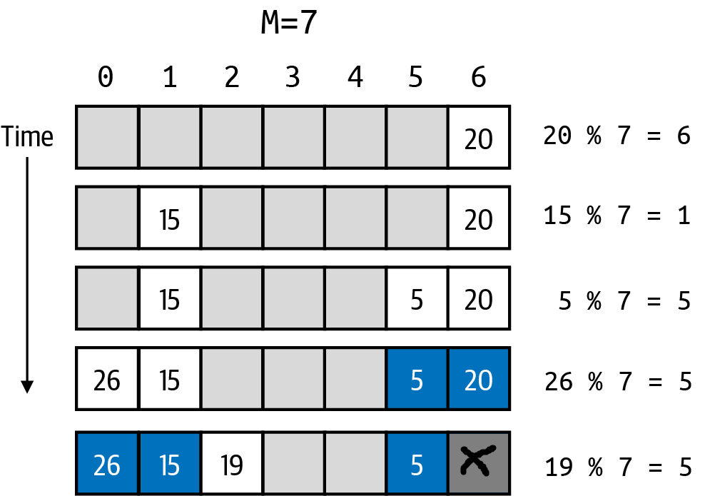
This means that you will not be able to "find" the key whose hash code was 19, and which appeared in index location 2 (because of wrap-around).

Can someone come up with an idea for a strategy for removing? Let’s discuss.

1.9 Comparison

It is instructive to compare performance with both of these approaches.

Assuming that you use geometric resizing when reaching a pre-determined "load limit", the resulting performance for put and get are O(1). Removing a value will yield a bit more work, but through similar analysis, you will find that it, too, is O(1).

What do you make of these graphs? The top one graphs, for each chain length, the total number of linked lists with that length.

First 10 values: [986, 4105, 8873, 12997, 14159, 12470, 9046, 5657, 2999, 1473, ...]

There are 986 empty indices, yielding a 98.7% utilization. The maximum chain is 16 and 4,105 are single (.1%).

The second grap also plots, for each chain length, the total number of index locations with that length.

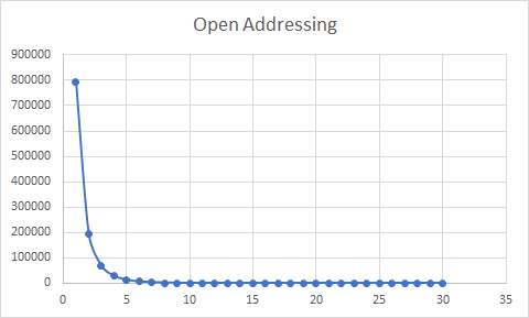
First 10 values: [792983, 195666, 69432, 28861, 13113, 6423, 3303, 1733, 977, 564, ...]

There are 792,983 empty indices, yielding a 28.8% utilization. The maximum chain is 34 and 195,666 are single (61%).

1.10 Interview Challenge

Each Friday I will post a sample interview challenge. During most technical interviews, you will likely be asked to solve a logical problem so the company can see how you think on your feet, and how you defend your answer.

You have three pair of colored dice – one red, one green and one blue – and for each colored pair of dice, one of the die is lighter than the other. You are told that all of the light dice weigh the same. And also you are told that all of the heavy dice weigh the same.

You have an accurate pan balance scale on which you can place any number of dice. The scale can determine whether the weight of the dice on one side is equal to, greater, or less than the weight of the dice on the other side.

Task: You are asked to identify the three lightest dice from this collection of six dice.

Obvious Solution: You could simply conduct three weight experiments.

1. Put one red die on the left pan, and the other red die on the right pan – this will identify the lighter red die

2. Put one green die on the left pan, and the other green die on the right pan – this will identify the lighter green die

3. 3. Put one blue die on the left pan, and the other blue die on the right pan – this will identify the lighter blue die This takes three weighing operations.

Challenge: Can you locate the three lighter dice with just two weight experiments, where you can place any number of dice on either side of the pan.

1.11 Version : 2023/04/07

(c) 2023, George T. Heineman