CS 2223 Apr 19 2022

Lecture Path: 21
Back Next

Expected reading: 515-527
Classical selection: Beethoven Symphony No. 2 (1802)

Visual Selection:

Musical Selection: UB40: Can’t Help Falling In Love (1993)

Visual Selection: The Starry Night, Vincent Van Gogh (1889)

Live Selection: White Rabbit, Jefferson Airplane, 1969

1 Graphs and Next Steps

A philosopher is a blind man in a dark room looking for a black cat that isn’t there. A theologian is the man who finds it.
H. L. Mencken

discussion...

1.1 Graphs

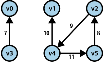
We are now studying a new domain in computer science called Graphs. A graph represents not just a set of items but the relationships between those items, which may be dynamically changed.

Figure 1:

Figure 2:

It is truly interesting to study graphs because there are several possible structures you can use to implement graphs, and there is no standardized solution that everyone agrees with.

Figure 3:

Start with some definitions:

A graph is a set of vertices and a collection of edges that each connect a pair of vertices.

Note that the graph is defined by a set of vertices; each vertex is therefore unique. Each vertex may have any number of edges (zero or more). However, it is common to avoid the following situations:

Self-loops: when a vertex has edge back to itself
parallel edges: when a vertex has multiple edges to the same paired vertex.

For our purposes, we will focus on simple graphs that avoid these two anomalies.

In this first lecture we are going to cover a number of new terms that are necessary to understand within the domain of graphs.

Vertex u is adjacent to vertex v if there exists an edge (u,v) in the graph.
A subgraph is a subset of a graph’s edges and the vertices that are connected to those edges.
A path is a sequence of vertices connected by edges.
A cycle is a path with at least one edge whose first and last vertices are the same.
The length of a path or a cycle is the number of edges in the path.
A graph is connected if there is a path from every vertex to every other vertex in the graph.

1.2 Trees

We have covered the Binary Tree structure in the context of Binary Search Trees, but when we come to graphs, the term Tree is a more generalized term.

A Tree is a graph that is fully connected and contains no cycles.

1.3 Structural Concerns

The vertices in a graph are essentially abstract concepts. For convenience, then, we simply refer to each vertex by 0, 1, ..., V-1 for a graph with V vertices.

For the algorithms we cover, we do not address situations where a vertex is added or removed; adding this capability doesn’t really change the complexity of the algorithms.

Naturally it becomes more convenient to have "names" or other arbitrary data associated with each vertex. To make this work, we will use the following standard:

SeparateChainingHashST<String,Integer> map = new SeparateChainingHashST<>(); SeparateChainingHashST<Integer,String> reverse = new SeparateChainingHashST<>();

map takes an arbitrary string and returns its associated vertex number (0, 1, ..., V-1) while reverse takes a given vertex number and returns its associated string. With these structures, we can retrieve (in ~ constant time) the necessary information for a vertex.

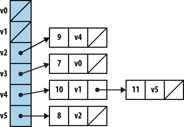
We can store a graph using any of the data structures we have seen so far. Two possibilities immediately come to mind:

Figure 4: Adjacency Matrix

Figure 5: Adjacency List

Which of these solutions is "best"? Well, it depends on the nature of the information you are storing

In 2012, Airports Council International (ACI) reported a total of 1,598 airports worldwide in 159 countries, resulting in a two-dimensional matrix with 2,553,604 entries. How many of these entries has a value? Well, that depends on the number of direct flights. ACI reported 79 million "aircraft movements" in 2012, roughly translating to a daily average of 215,887 flights. Even if all of these flights represented an actual direct flight between two unique airports (clearly the number of direct flights will be much smaller), this means the matrix is 92% empty. This is a good example of a sparse graph.

A complete graph is one where there is an edge between a vertex and every other vertex in the graph.

Since there could be on the order of V*(V+1)/2 possible edges in a graph with V vertices, then in a dense graph, the number of edges is proportional to the square of the number of vertices. In a sparse graph, the number of edges is proportional to the number of vertices.

1.4 Mathematical Analysis

When analyzing graphs and graph algorithms, we will typically use two variables in our formulae:

V – The number of Vertices
E – The number of Edges

And often the performance of a specific algorithm will improve (or degrade) based on whether a graph is sparse or dense.

1.5 Processing Graph Queries: Search Triangles

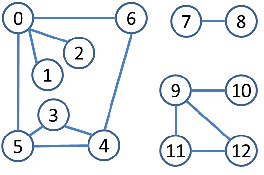
Let’s get started with a simple request. Given the above graph, can you find all Triangles that exist, namely, three vertices u, v and w in which all three edges (u,v), (v,w) and (u,w) exist and these vertices are all different.

Let’s brainstorm for a bit. How would you imagine doing this? How would you make sure that you don’t double count the number of triangles that you see?

Sample code FindTriangle contains different variations on this problem. The basic premise looks like this:

for (int u = 0; u < g.V(); u++) { // for all vertices u... for (Integer v : g.adj(u)) { // find a neighbor v to u for (Integer w : g.adj(v)) { // then find neighbor w to v for (Integer x : g.adj(u)) { // and check if w is neighbor to u if (x == w) { // Triangle } } } } }

The above will overcount the number of triangles and so you need to divide the toal number found by 6, since there are 3! permutations of each of the vertices.

This triangle finding example is rather specific and we likely need some more generic searching capability. This week we cover a number of graph searching algorithms to address this very question.

Doesn’t match: Expected Results when using (x == w) because of Java’s default equality implementation. When you change this statement to become x.equals(w) it works!

This is going to take awhile! Also: results do not match published expectation. N E CountE CountT Est. 8 15 14 8 7.0 16 66 60 96 70.0 32 257 248 669 620.0 64 1008 1008 5087 5208.0 128 4075 4064 42921 42672.0 256 16242 16320 44317 345440.0 512 65538 65408 40371 2779840.0 1024 261599 261888 42432 2.2304128E7

1.6 Working with graphs

I want to start by considering the fundamental operations for graphs as shown in the following table:

public class	Graph
	Graph(int V)	create graph with V vertices an no edges
	Graph(In in)	load graph from input
int	V()	number of vertices
int	E()	number of edges
void	addEdge(v,w)	add v-w to graph
Iterable<Integer>	adj(int v)	vertices adjacent to v
String	toString()	string representation

As we will see, you can implement a wide variety of algorithms simply by working with this Graph API. Now there are two proposed strategies for storing graphs.

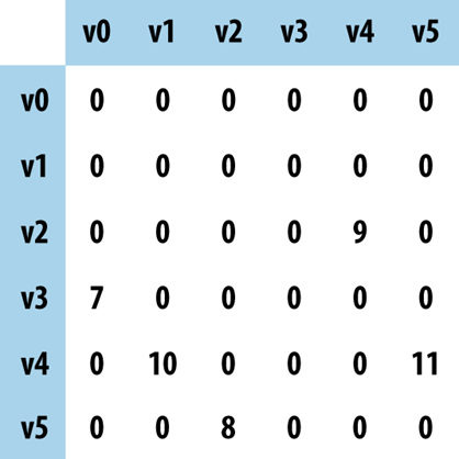
Adjacency Matrix – Use a V-by-V boolean two dimensional array where entry [v][w] determines whether there is an edge from v to w. Space is prohibitive and would be useful only for very dense graphs.
Array of Adjacency Lists – Use a one-dimensional vector of size V to record the collection of edges that are adjacent to each vertex. In an undirected graph, each edge appears twice.

We will work in lecture using the Adjacency Lists implementation and you will get a chance to see the Adjacency Matrix implementation on a homework assignment.

As summarized on page 527, the order of growth performance for each of the graph implementations is as follows:

Comparison	Adjacency Matrix	Adjacency lists
space	V2	E + V
add edge v-w	1	1
check w adjacent to v	1	degree(v)
iterate vertices adjacent to v	V	degree(v)

Adjacency matrices have excessive space costs and unexpectedly high cost to iterate over neighbors of v.

1.7 Constructing Graphs

It is not as convenient to work with graphs because it takes so long to set them up "from scratch". It is common to store information in a file and load it up to instantiate the graph. On page 529 of the book there is an example file tinyG.txt which contains the following:

13 13 0 5 4 3 0 1 9 12 6 4 5 4 0 2 11 12 9 10 0 6 7 8 9 11 5 3

I created a class, GraphLoader to easily load up a graph file from disk. The format is Sedgewick’s own.

The first line shows the number of nodes (in this case 13). The second line shows the number of edges (oddly enough, 13 again). Then the next 13 lines all contain a single edge described by two integers representing the vertices in the graph.

When a Graph is constructed from this file, the following is the result.

The following shows the adjacency matrix representation for this graph.

00 01 02 03 04 05 06 07 08 09 10 11 12 00 1 1 1 1 01 1 02 1 03 1 1 04 1 1 1 05 1 1 1 06 1 1 07 1 08 1 09 1 1 1 10 1 11 1 1 12 1 1

1.8 Processing Graph Queries: More general

There are a number of common queries that you would have given a graph structure. The most common is based on reachability, namely, can you start at a given vertex v and find a path to another vertex w. And you must perform this computation as efficiently as possible.

1.9 Search Graphs

To motivate searching over graphs, consider the following maze:

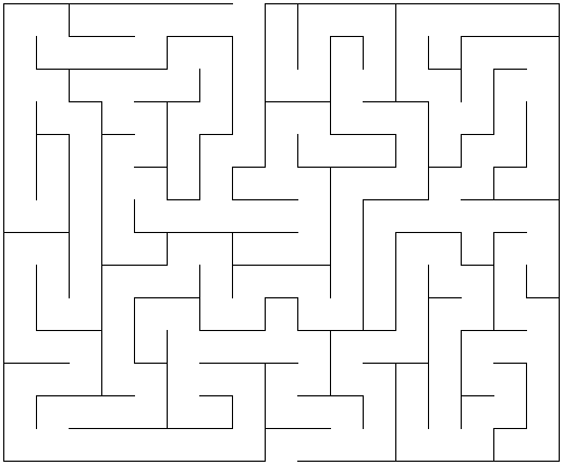
Think about how you solve this maze. For the purpose of this course, let’s represent the maze as a graph. I only show a fragment of this construction:

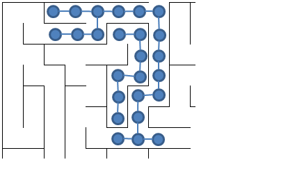
In computer science we routinely transform problems; in this case, we are going to solve a maze by transforming it into a graph of NxM vertices (one for every positions in the N rows and M columns. An edge in the graph exists if two positions are neighbors with no wall between them. This is an example of a sparse graph.

1.10 Initial Approach to Searching a Graph

Let’s use some intuition to construct our first algorithm for searching through a graph. If only we had some way to keep track of our progress! Let’s imagine marking nodes that we have already seen.

Unusual for class constructor to do any work. This is how Sedgewick implements graphs, so I will keep it as well.

public DepthFirstSearch (Graph g, int s) { marked = new boolean[g.V()]; this.g = g; dfs(s); } /** Continue DFS search over graph by visiting vertex v. */ void dfs (int v) { marked[v] = true; // we have now seen this vertex count++; // look into neighbors for (int w : g.adj(v)) { if (!marked[w]) { // will never dfs() on this vertex again dfs (w); } } }

This proceeds until all vertices reachable from the initial vertex s have been processed.

For any handwritten exercises, I will always process neighbors in ascending order of their vertex identifiers.

Now, in what order are the vertices processed? It depends on the way they are traversed with the for (int w: g.adj(v)) code. And the order unfortunately depends upon the way that the adjacency list stores the neighbors.

Since we are using a Bag to store the vertices, we have no way to know what this ordering will be. But does it really matter? Since this is a blind search the answer is no!

However, when we work on examples in class or perhaps on an exam, I will always assume that neighboring vertices are iterated in ascending order based upon their unique identifier.

1.11 Demonstrate DepthFirstSearch

Demonstrate using Shell and running DepthFirstSearch on the files tinyG.txt and tinyCG.txt.

There are several observations to make:

The number of invocations of dfs will also be ≤ V.
Each edge (u,v) is visited twice, once as a neighbor of u, and once as a neighbor of v.
The Depth of the recursion ≤ V.

1.12 Recovering Path

This small search utility demonstrates the behavior of Depth First Search, but it doesn’t really do much. Let’s add behavior to recover the path from a designated vertex, s, to any vertex that is reachable from s over the existing edges in a graph.

At first it seems we have to keep track of a lot of information, because there are so many directions in which the search might go. However, instead of thinking about the starting point of an arrow, focus on the ending point of the arrow.

Recovering the path will be fully described tomorrow.

The counter-intuitive solution to this problem is to record a separate one-dimensional vector for each vertex that records the previous vertex in a depth first search from the original s source vertex.

1.13 Sample Exam Question

You are given the following graph. Assuming that all adjacency lists are ordered by increasing vertex number, conduct a depth first search of the graph starting at vertex 0 and stopping when you reach vertex 7.

Show your progress by coloring completed vertices in Black while marking in-progress vertices with an X.

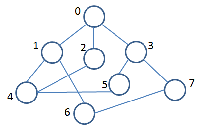
Find fully worked out step-by-step answer in Canvas under Files | handouts | day21_DFS_StepByStep

1.14 Daily Question

What happens to Depth First Search if the graph is not connected?