CS 2223 Apr 23 2021

Lecture Path: 18
Back Next

Expected reading:

Classical selection: Rachmaninoff Piano Concerto no. 3 in D-minor, (1910)

Visual Selection:

Musical Selection: Centerfield, John Fogerty (1985)

Visual Selection: The Dance Class, Edgar Degas (1874)

Live Selection: Bruce Springsteen The Promised Land (1980)

1 Self-Balancing Binary Trees

For this lecture, we are now viewing a Binary Search Tree as containing just Keys. This simplifies the method signatures of the related calls.

This also implies that multiple nodes can exist in the BST with the same key. These duplicate values are perfectly fine, since the BST is know just maintaining a collection of vlaues that are inserted or deleted.

1.1 Getting Started

To get started, conduct a post-order traversal of the following tree. That would look like the following:

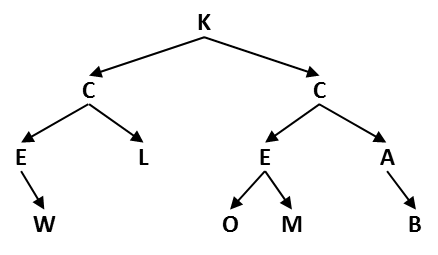
Is this a proper BST?

1.2 Homework3

There were some updates to the description for HW3. Please pay attention to them. In particular, Q3.1 and Q3.2 are actually bonus questions. The real question is to find the outlier play.

Check the rubric if you have questions.

1.3 Balanced Trees

Today we will discuss how to automatically balance Binary Search Trees so they retain their efficiency.

It is easy to see that a BST can become out of balance. Just consider adding three values to a tree in descending order, such as 50, 30, and 10. The resulting tree skews to the left as shown below:

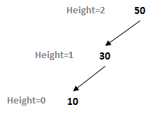
One way to describe this skew is to identify two paths from the root to any root, whose lengths are noticeably different. Here, there is a path of length 2 from 50 - 30 - 10, and there is also a path of length 0 from 50 to the right (note there is no right child of root).

Once again, note how the height of a node in a BST is computed based on the maximum distance from that node to any of its descendants. Thus a binary tree with a single root node (with no children) would have height zero.

A balanced tree for these same values would look like the following:

At a glance it looks quite different, but if you inspect its internal structure you can see there is a similarity. Indeed, let’s fill in some values and see if there is a pattern of behavior that we can exploit.

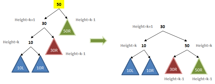
In this extended example, the BST has additional nodes, and the colored triangles describe collections of values. Note that the root node has a left subtree whose height is k+1 while its right subtree has a height of k-1. Having just this small imbalance is enough to begin the process of degrading the overall performance.

The technique of self-balancing a tree was discovered in 1962 by Adel’son-Vel’skii and Landis and it first appeared in a Russian mathematical journal. In CS this balancing binary search tree is known as an AVL tree.

An AVL Tree guarantees the AVL Property, namely, that the height difference for any node is -1, 0 or +1.

Assuming the above property holds, then the AVL tree is considered to be balanced. An AVL tree can become unbalanced by inserting or removing values from the tree. So you need to take care to properly correct whenever you observe that the tree has become unbalanced.

Remember the first time I introduced the BST that each node maintained an attribute, N, that reflected the number of values in the subtree rooted at that node? The original BST code had to properly compute N as each recursive invocation completed.

We will do the same thing. Upon observing an unbalanced node somewhere in the BST, special logic will be introduced that will correct the imbalance according to the AVL Property.

1.4 Delete

If you are curious, a different delete implementation is provided, called fastDelete in the AVL tree.

AVL

1.5 Four Scenarios

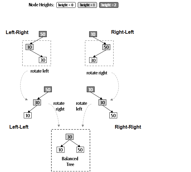
Given three values to be inserted into a BST, there are four imbalanced scenarios that need to be considered:

Each of these has a label associated with it that explains how to correct the imbalance. The case we covered earlier is Left-Left because of the relationship between these three values.

RotateRight operation

Let’s define an operation on a Binary Tree node called Rotate Right which adjusts the relative heights to conform to AVL. In this example, we can "lift" up 30 to effectively replace 50 as the root, and 50 is demoted to be a right child of 30.

Regardless of where the 50 node exists within a BST, the rotate right operation will properly rebalance the tree below it to conform to the AVL property. Naturally you have to continue working back up to the root as the recursion unwinds to make sure that successive ancestors also remain balanced. Fortunately on insert you only need one rotation to bring the tree back into balance. When deleting values, you may also have to rebalance, and in that case you may need multiple rounds of rebalancing.

As you can see from the sample code, each rotation operation is a fixed number of operations, so it can be considered to be constant. Since the height is now guaranteed to be ~log N, we have delivered on our promise for efficient BST data structures.

Let’s cover one of the more complicated examples, namely the Left-Right scenario. It isn’t enough to conduct a single rotation; you actually have to do two rotations:

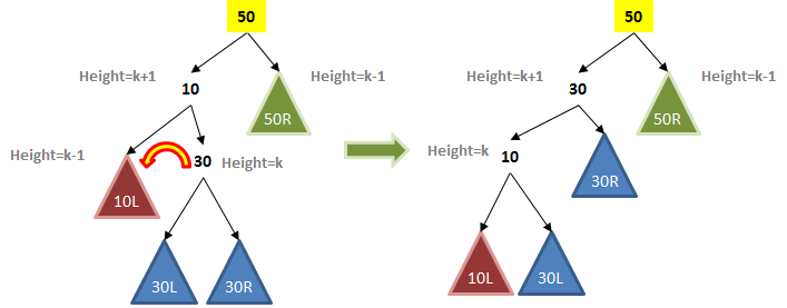
As you can imagine, first a left rotation is performed to move the 30 up and the 10 down. Then a Right rotation is performed to lift the 30 up and move the 50 down. All corresponding subtrees are also adjusted.

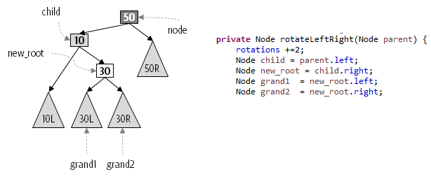
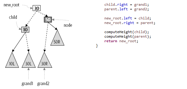
The key to efficient AVL implementation is that each node stores its height value so it doesn’t have to be computed each time.

1.5.1 Red Black Trees

The Red Black Tree as described in pp. 424-437 is excellent. To be honest, this was the first time that I was able to fully understand Red Black trees. The key points you need to understand are:

AVL trees enforce a strong global property, namely, that the heights for left and right subtrees are never more than -1, 0 or 1. If you relax this restriction, you can reduce the number of rotations.
A RedBlack tree guarantees that no path to a leaf node is more than twice as long as any other path to another leaf node. This is strong enough to guarantee the desired properties.
RedBlack trees therefore allow for less compact trees, which increases the search time slightly, but it noticeably reduces the time to perform insertions and deletions.

1.6 Demonstration

Run some comparisons. AVL is implementation I provide. RedBlack is simplified coding as provided by Sedgewick in book which is easy to understand, though not as efficient as possible.

TreeMap is the highly optimized implementation of java.util.TreeMap that outperforms most implementations, especially with regards to speed.

Average Number Of Rotations N AVL RedBlack TreeMap 8 0.125 0.5 0.0 16 0.187 1.5 0.187 32 0.375 2.218 0.281 64 0.359 3.109 0.218 128 0.382 4.492 0.359 256 0.371 5.214 0.371 512 0.359 6.632 0.382 1024 0.356 7.757 0.350 2048 0.356 8.759 0.361 4096 0.376 10.18 0.371 8192 0.372 11.65 0.377 16384 0.371 12.675 0.379 Height of Resulting BST N AVL RedBLack TreeMap 8 3 3 3 16 4 4 4 32 5 6 5 64 6 7 6 128 7 9 7 256 9 10 9 512 10 11 10 1024 11 13 11 2048 12 14 12 4096 13 16 14 8192 15 17 15 16384 16 19 16

Finally, what if we just insert the numbers from 1 to N in ascending order, which would otherwise produce the worst behavior.

N A-Ht. RB-Ht. TM-Ht. 7 3 3 4 15 4 4 6 31 5 5 8 63 6 6 10 127 7 7 12 255 8 8 14 511 9 9 16 1023 10 10 18 2047 11 11 20 4095 12 12 22 8191 13 13 24 16383 14 14 26 32767 15 15 28 65535 16 16 30 131071 17 17 32

1.7 Sample Exam Questions

The first question is suitable for a True/False:

In a binary tree with N nodes, there must be at least n/2 leaf nodes.

1.8 Daily Question

Find the daily question in Canvas to answer.

1.9 Interview Challenge Exercise

Write a method for a Binary Search Tree that returns the Key for the node that has the greatest depth: that is, the node that is the farthest from the root node. If there are multiple nodes that share this same distance, then print any one of them.

Given the BST that results from a straight-forward assembly using the words in order from new ShakespearePlay(7), what is the key of greatest depth?

Email or discord me the answer and you get a prize!