The term optimization is a misnomer. The problem of changing code in all cases to the best it can be is an undecidable problem; it cannot be solved an algorithm on a computer.

We can, however, improve code in most cases.

There are machine dependent optimizations such as good allocation of registers and machine independent optimizations such as computing constants; constant computation at compile-time rather than generating code to compute them saves execution time.

Optimization can consume a lot of compile-time, so we want the most payoff for the least effort. In particular, the compiler needs to guess where the most frequently executed parts of the program are.

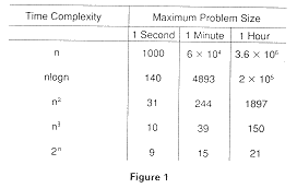
If we let S = problem size, then after a speed-up by a factor of 10:

 

 	Complexity		Problems Size

 

 	Linear (n)		10S

 	nlogn 			10S (for large S)

 	n2 			3.16S

 	n3 			2.15S

 	2n 			S + 3.3

 

We can conclude from this that bad algorithms are not helped much by optimization.

However, clever optimizations of clever code may not improve things either. Knuth (1971) presented an amusing discussion in which he referred to an algorithm which he had developed many years ago which translated a complicated expression to fewer instructions than some other people's algorithm. Years later, he realized that programmers rarely used such complicated expressions, and it isn't worth the compiler's time to optimize them.

For (1), Knuth (1971) shows empirically that simple assignment statements with one operation and one to three variables are themost often used statements:

 	A := B 	A := A OP 1 	A := A OP k 	A := B OP k 	A := B OP C 

For (2), code in loops tends to be executed the most; thus optimizations concentrate onloops.

Principle 1. If you can't do it safely, don't do it.

Principle 2. Don't expect the programmer to optimize high-level language features.

 EXAMPLE 1 Two-dimensional arrays

 	LOOP

 	  A[I,J] := . . .

 	  . . .

 	  . . .

 	   := A[I,J]

 	  . . .

 	ENDLOOP

 

The translated code for Example 1 quite likely has "things" which can be optimized. The programmer could conceivably do it -- By using one-dimensional arrays, etc. Realistically, then, the programmer might as well not be using a high-level language.

---

Optimizations optimize most frequently for time. This is represented, syntactically (that is, it can be seen by looking at the code), by minimization of the number of operations and minimization of the number of memory accesses. Operations can be computed faster if their operands are in registers. Constants can be computed at compile-time.

Optimizations optimize next most frequently for space . Minimizing memory accesses may produce a smaller amount of code as well as code that executes faster since most machine code requires more bytes to reference memory.

There are also space-time tradeoffs. For example, replacing two instances of the same code by a subroutine may save code space, but takes more time because of the overhead of jumping to the subroutine, passing arguments and returning from the subroutine.

An optimization should speed up a program by a measurable amount. Also, we don't optimize in heavy debugging environments (student environments are heavy debugging environments). It takes too much compiler time for environments where a program is compiled many times (until it is correct) and run once or twice.

On the other hand, as we shall see, certain so-called peephole optimizations are so easy that they should be done by all compilers.

The phase which represents the pertinent, possible flow of control is often called control flow analysis. If this representation is graphical, then a flow graph depicts all possible execution paths. Control flow analysis simplifies the data flow analysis. Data flow analysis is the proces of collecting information about the modification, preservation , and use of program "quantities"-- usually variables and expressions.

Once control flow analysis and data flow analysis have been done, the next phase, the improvement phase, improves the program code so that it runs faster or uses less space. This phase is sometimes termed optimization. Thus, the term optimization is used for this final code improvement, as well as for the entire process which includes control flow analysis and data flow analysis.

Optimization algorithms attempt to remove useless code, eliminate redundant expressions, move invariant computations out of loops, etc.

The next section describes control flow analysis. We begin by creating the control flow graph.

Leaders

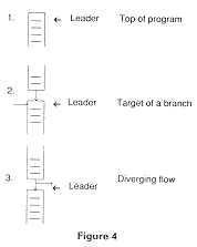
A basic block consists of a leader and all code before the next leader. We define a leader to be (1) the first statement in the program (or procedure), (2) the target of a branch, identified most easily because it has a label, and (3) the statement after a "diverging flow " : the statement after a conditional or unconditional branch. Figure 4 shows this pictorially:

Since a basic block consists of straight-line code, it computes a set of expressions. Many optimizations are really transformations applied to basic blocks and to sequences of basic blocks.

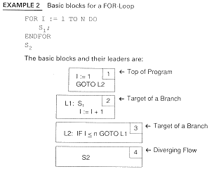
Although this program might be translated in different ways, the discussion here is still valid.

Formally, a flow graph is a directed graph G, with N nodes and E edges. (Remember that a directed graph is a connected set of nodes where every node is reachable from the initial node.) Example 3 shows the control flow graph for Example 2. The rules for building such a graph follow.

In Example 3, we see that the set of nodes is the set of basic blocks and the set of edges is determined by looking at places where the nodes branch.

---

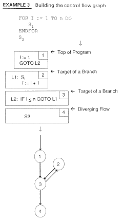
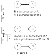
Building a control flow graph involves finding predecessors and successors.

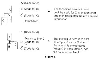
Consider the first situation of Figure 6 where basic block A has been built and a leader is identified for the beginning of basic block B. We cannot build the tail of the arrow to basic block B until we find the diverging flow that leads here. Backpatching: returning and filling in the tail information, will define the source of this arc.

The second picture represents the opposite situation. In the second picture in Figure 6, we know we have an arc, but haven't found the leader to which the arc should point; the tail of the arc is known, but its head is not. Here, we can allocate a data structure for a basic block and then backpatch when it is found.

Basic blocks may be created and destroyed as the program is modified in the optimization process. Thus, space must be made available for growing collections of blocks. Storage reclamation is essential to handle optimization of large programs.

Since the structure of the flow graph varies with time, the data structure for blocks might keep pointers to lists of successors.

Since statements within the block change with time, it is reasonable to keep the intermediate representation as a linked list and reclaim storage of unused statements. Another possibility is to allocate dynamically on a heap and then garbage collect (see a data structures text if the terms heap and garbage collection are not familiar) when the heap runs out. See Module 12 for a discussion of garbage collection.

The previous sections looked at the control flow graph nodes of basic blocks. DAGs, on the other hands, create a useful structure for the intermediate representation within the basic blocks.

A directed graph with no cycles, called a DAG (Directed Acyclic Graph), is used to represent a basic block. Thus, the nodes of a flow graph are themselves graphs!

We can create a DAG instead of an abstract syntax tree by modifying the operations for constructing the nodes. If the node already exists, the operation returns a pointer to the existing node. Example 4 shows this for the two-line assignment statement example.

In Example 4, there are two references to a and two references to the quantity bb * 12 .

---

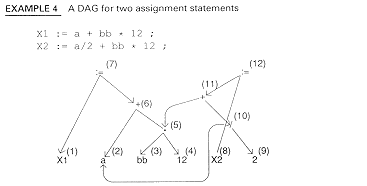
As Example 4 shows, each node may have more than one pointer to it. We can represent a DAG internally by a process known as value-numbering . Each node is numbered and this number is entered whenever this node is reused. This is shown in Example 5.

 EXAMPLE 5 Value-numbering

 

 	Node	   Left Child	    Right Child

 	1. X1

 	2. a

 	3. bb

 	4. 12

 	5. * 		(3)		(4)

 	6. +		(2)		(5)

 	8.y :=		(1)		(6)

 	8. X2

 	9. 2

 	10. /		(2)		(9)

 	11. +		(10)		(5)

 	12. :=		(8)		(11)

 

When a DAG is created, common subexpressions are detected. Also, creating a DAG makes it easy to see variables and expressions which are used or defined within a block.

DAGs also produce good code at code generation time. In Module 11, we will see a code generation algorithm which produces good (but not optimal!) code from a DAG.

Example 6 shows a bubble sort procedure and a set of quadruples to which it might be translated. Quadruples are an intermediate representation consisting of a single operation, up to two operands and a result. They are easier for humans to read than an abstract syntax tree. The quadruples shown here are in "assignment statement" form.

 EXAMPLE 6 IR for a bubble sort procedure

 	FOR I := 1 TO n - 1 DO

 	        FOR J := 1 TO I DO

 		IF A[J] > A[J+1] THEN

 		    BEGIN

 			Temp := A[J]

 			A[J] := A[ J + 1 ]

 			A[ J + 1 ] := Temp

 		    END

 
 	
 		

 		I := 1

 		GOTO ITest

 	ILoop:	J := 1

 		GOTO JTest

 	JLoop:	T1 := 4 * J

 		T2 := A [T1] 		; A[J]

 		T3 := J + 1

 		T4 := 4 * T3

 		T5 := A[T4] 		; A[ J + 1 ]

 		IF T2 <= T5 GOTO JPlus

 		T6 := 4 * J

 		Temp := A[T6] 		; Temp := A[J]

 		T7 := J + 1

 		T8 := 4 * T7

 		T9 := A[T8] 		; A { J + 1 ]

 		T10 := 4 * J

 		A[T10] := T9 		; A[J] := A[ J + 1 ]

 		T11 := J + 1

 		T12 := 4 * T11

 		A[T12] := Temp		; A [ J + 1 ] := Temp

 	JPlus:	J := J + 1

 	JTest:	IF J < = I GOTO JLoop

 	IPlus:	I := I + 1

 	ITest:	IF I <= n - 1 GOTO ILoop

 

The intermediate code shown in Example 6 is rather high-level. For machines which have no indexing modes, the references to A[...] will have to be computed by the compiler. Also, the IF statements really involve several quadruples (see Module 6). The multiplication by "4" could, alternatively, be done at code generation time. We do it here because it will give us more opportunities for optimization of our example.

Using "( )" to mean "contents of " and "addr" to mean "address of", the low-level quadruples for "Temp := List[i]" might be:

 	T1 := addr(List)

 	T2 := T1 + I

 	temp := (T2)

 

Similarly, if the array reference is on the left-hand side of an assignment statement as in "List[i] := temp", low-level quadruples would be:

 	T1 := addr (List)

 	T2 := T1 + I

 	(T2) := Temp

 

Even if a machine has an indexing addressing mode, translating array references into their low-level format may allow optimizations (for example, if the subscript reference were a common subexpression).

Nevertheless, there will be numerous opportunities to improve the code sequence in Example 6.

---

The program of Example 7 contains cycles which may be loops. Determining loops is a major activity of control flow analysis. Creating basic blocks and a control flow graph are two steps toward this process. In the next section, we will formalize the process of determining a loop in a control flow graph.

---

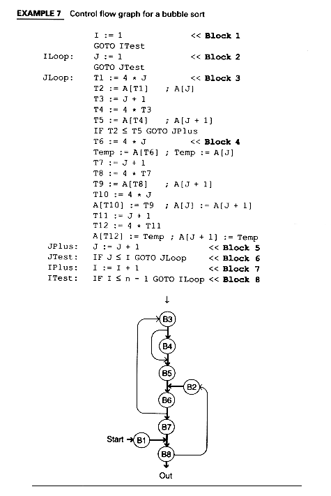
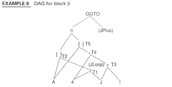
There are two main types of loop optimizations: (1) movement of loop-invariant computations outside of the loop and (2) elimination of excess induction variables, the variables which are a linear function of the loop index. Other optimizations often performed within loops are reductions in strength of certain multiplications to additions.

Example 9 shows invariant code movement. The details of how this optimization is found and implemented are given in the next two modules. In this module we focus on the importance of being able to identify a loop.

EXAMPLE 9 Invariant code motion

 	FOR index := 1 TO 10000 DO	t := y * z

 	BEGIN				FOR index := 1 TO 10000 DO

 		x := y * z ;		BEGIN

 		j := index * 3 ; -- >		x := t

 	END					j := index * 3

 	.				END

 	.				.

 					.

 

In Example 9, y * z is computed each time around the loop. If none of y, z, or x changes value in the loop (and this must be checked!), then it is more efficient to compute this product, t, one and to use t every place the computation appears in the loop (x itself may be able to be be eliminated).

Example 9 can also be optimized for strength reduction (turn the multiplication into an addition) and for elimination of induction variables (index and j are tracking one another). We will save these examples for Module 10.

---

8.6.1 Defining a Loop

Intuitively, cycles in flow graphs are loops, but to perform optimizations we need a second property:

A loop must have a single entry point

A cycle must have a header to be considered a loop. Optimizations such as code motion cannot be done safely if there is more than one entry to the loop. Also, the header concept makes the algorithms for loop-invariant code motion, etc. conceptually simplier.

Example 10 shows a flow graph with two cycles, one of which is a loop and one of which is not a loop.

Although the preceding definition is helpful for us humans to find a loop, we will need some more definitions in order to write an algorithm to find a loop.

An efficient algorithm for finding a loop involves finding dominators, depth-first search, and depth-first ordering.

Here, the start node dominates all nodes; Node A and Node B do not dominate anything except themselves, Node C dominates Node D and itself, and Node D does not dominate anything except itself.

---

Algorithm

Finding Dominators

 DOM (Start) := {Start}

 FOR node < > Start DO

 	DOM (node) = {All nodes}

 ENDFOR

 WHILE changes to any DOM(node) occur DO

 	FOR each node < > start DO

 		DOM(node) = {node}  (  Dom(p) )

 				      p  Pred(node)

 	ENDFOR

 ENDWHILE

 

there must be a least one arc entering the header from a node in the loop

The natural loop of the back edge is defined to be the smallest set of nodes that includes the back edge and has no predecessors outside the set except for the predecessor of the header. Natural loops are the loops for which we find optimizations.

Algorithm

Finding the nodes in a natural loop

FOR every node n, find all m such that n DOM m
FOR every back edge th, i.e., for every arc such that h DOM t, construct the natural loop:


Delete h and find all nodes which can lead to t

These nodes plus h form the natural loop of th

A depth-first order is defined to be the reverse of the order in which we last visit the nodes of the control graph when we create the DFST. The following algorithm creates a depth-first spanning tree.

Algorithm

DFST

 T := empty

 n := Start node

 REPEAT

 	IF n has an unmarked successor s THEN

 	BEGIN

 		Add n  s to T

 		Mark s

 		n := s

 	END

 	ELSE

 		n := parent of n in T

 UNTIL n = start node and n has no unmarked successors

 



---

We introduce one more definition - a backwards edge.

To find the loops of a program efficiently:
1. Compute a depth-first order (DFO). The backwards edges are those whose heads precede their tails in the DFO.

2. Compute Dominators. The back edges are the backwards edges whose heads dominate their tails.

3. For each back edge, compute the natural loop.