[WPI] [cs2223] [cs2223 text] [News] [Syllabus] [Exams] [Exam 4] 

cs2223, D97/98 Exam 4 Solution

Question 4.1

The first algorithm makes each dot either black or white with a 50% probability. The average gray level in a picture element is 0.5 and the dots are as uniform as the random generator. This algorithm addressed each locationin the array so the number of operations - calls to rand(), number of accesses to picture[][], etc are all O(N) where

In the first algorithm, the number of picture elements painted black is about N/2 but it can vary because of randomness.

The second algorithm picks random locations (one half the number of elements in the array) and puts the black value in them. So, there are exactly N/2 picture elemtens painted black. However, because of the possibility that some locations are written more than once - which doesn't make the picture elements any darker - the actual number of black picture elements - and thus the overall average gray level might be lower than for the first algorithm.

Look at a single element. The probability that it gets any one of the hits is:

Thus the probability that it doesn't get the hit - and it stays white - is

The probability that the picture element stays white after two hits is the square of this:

The probability that the picture element is still white after all N/2 hits is

The probability that the picture element is black after all N/2 hits is one minus this.

This, times the "black" level (1.0) is the average gray level for a picture element. And it is less than 0.5.

The second algorithm is also of order O(N). The number of calls to rand() is N and the number of accesses to the array picture[][] is N/2. So the functions have the same order and produce similar results - although the second produces a less dark image than the first. There is no clear case for either algorithm being superior.

If you wondering about the numerical value of the above expression, the enclosed spreadsheet shows that its asymptotic value is 0.393469. Note, a zip versionis available for those whose browsers do not allow downloading Excel files. The enclosed script shows a numerical simulation using the two functions gray1() and gray2(). The simulation values match the values calculated above.

Question 4.2

The hard way to do these problems is to modify the N-queens algorithm discussed in Section 9.6.2 of the text and in Class 26. The modifications include:

For the N-rooks problem, there is no need to make the 45° and 135° tests.

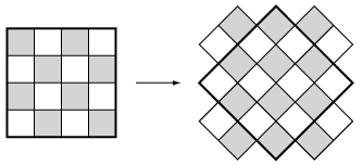
For the N-bishops problem, the approach has to be changed. Now the colun vector approach cannot be used because any number of bishops can be in the same row or column. One way to modify the problemso thatwe can use the N-queens code is to rotate the chessboard by 45°. Thus a NxN chessboard becomes a (2N-1)x(2N-1) chessboard. Now rows and columns interchange and the solution canbe found using the code for the N-rooks problem. Don't forget to eliminate any solutions which try to put bishops in the "corners" of the rotated chessboard.

The easier way to solve this problem is to notice the methods we restricted the solutions to those with no chess pieces in the same rows and columns.

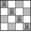
There can be no more than N rooks because each occupies one row or column. One solutionis to place them all on a diagonal:

That is an algorithm.

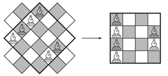
From the "rotated chessboard" image above, it would seem that we should be able to place as many as (2N-1) bishops. So we place one per "row" of the rotated chessboard as close to the corners as possible. And, we have to eliminate the final bishop because it will reside on the same "column" as the first. Here is a way to place the (2N-2) bishops - fill up one edge and fill the opposite edge except for the two corners.

That is an algorithm.

Question 4.3

There are many ways to solve this problem. This one follows nodeA back to the root, storing the pointers in an array. Then the pointers beginning at nodeB and back to the root are compared with each of the elements in the array. The matching value is returned.

node *nearest_ancestor(node *nodeA, node *nodeB)
   {
   vector <node *> node_list; // an array to hold pointers to nodes
   node_list.resize(BIG_ENOUGH) // the max possible depth of the tree
   node *temp; // a temporary pointer
   int node_count = 0; // to count the number of nodes
   
   for (temp = nodeA; temp; temp = temp.parent) // loop upward to the root
      node_list[node_count++] = temp; // add the node to the array
      
   // the array now contains the path from nodeA to the root
   
   for (temp = nodeB; temp; temp = temp.parent) // loop upward to the root
      {
      for (int i = 0; i < node_count; i++) // loop through array
         if (temp == node_list[i]) return temp // found it
      }
   return 0; // If this command executes, something has gone wrong
   }

Here is another implementation of the same algorithm:

node *nearest_ancestor(node *nodeA, node *nodeB)
   {
   for (node *p2a = nodeA; p2a; p2a = p2a.parent) // loop upward to the root
      for (node *p2b = nodeB; p2b; p2b = p2b.parent) // loop upward to the root
         if (p2a == p2b) return p2a; // found it
   return 0; // If this command executes, something has gone wrong
   }

If the array is complete, its depth is. You can show that by using the same analysis as we showed in Class 8. Then it takessteps to fill the array andsteps to compare the values looking for a match. This is the order of this algorithm.

More efficient algorithms exist. For example, we can store both paths in arrays and sort the arrays. We then use a merge-sort technique until the match if found. Creating the arrays is of orderand sorting them is of order, which is the order of the algorithm.

The grading criteria are available. These are subject to interpretation by the grader. As we stated in class, our primary goal in the grading of these exams is consistency. If your intrepretation differs from the grader's and the grader has applied her/his criteria uniformly, then the grader's interpretation will prevail.

[cs2223 text] [News] [Syllabus] [Exams] [Exam 4]

Contents ©1994-1998, Norman Wittels
Updated 30Apr98