cs2223 Class 15

[WPI] [cs2223] [cs2223 text] [News] [Syllabus] [Classes]

cs2223, D97/98 Class 15

Analysis of Divide and Conquer Algorithms

We discussed two divide and conquer sorting algorithms and analyzed their efficiency.

Merge Sort

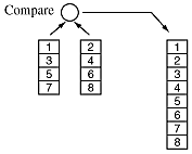
Suppose we have two already-sorted sub-arrays of size N/2. We can combine them by comparing the top numbers, one at a time in pairs, and adding the smallest to a new array of size N.

Figure showing two stacks. The top-most elements - the ones which would be popped next - are being compared to decide which is smaller and should be pushed on to a third stack.

This operation is inherently recursive. An array of size N is split into two arrays of size N/2, which are recursively halved again and again. When the sub array sizes are one, a simple comparison between two numbers is made. There are many details involved in writing code for this algorithm - how to dynamically allocate and deallocate all of the subarrays, how to handle arrays whose sizes are not powers of two, etc. We will ignore these details and analyze the simple case when N is a power of two.

Let's calculate the number of binary comparisons required to merge sort an array of size N. Note, right away, that the best and worst cases are the same. There is no arrangement of the numbers in the array which will increase or decrease the number of comparisons. So, our calculation will probably be correct for best, worst, and average cases.

Notice that N-1 comparisons are required to sort the two sub arrays of size N/2 since the last number doesn't have to be compared - it automatically goes at the end of the merged array. This is in addition to the number of comparisons required to sort the two arrays of size N/2. The recurrence relation for the number of comparisons is:

The initial condition states that an array with only one number requires no comparisons. This recurrence relation can be solved using the substitution we introduced in Class 8 and the Method of Undetermined Coefficients from the Recurrence Relation Notes.

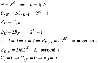
N = 2^K --> K = lg(N); C(2^K) - 2*C(2^(K-1)) = 2^K =1; B(K) defined as C(2^K); B(K) - 2*B(K-1) = 2^K -1; x - 2 = 0 --> x = 2 --> B(K; homogeneous) = A*2^K; B(K; particular) = D*K*2^K + E; C(1) = 0 --> C(2^0) = 0 --> B(0) = 0

The factor of K in the particular solution is because of the repeated root - 2^K is already part of the homogenous solution. Solve for D and E by substituting the particular solution back into the recurrence relation:

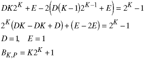
D*K*2^K + E - 2*(D*(K-1)*2^(K-1) + E) = 2^K -1; 2^K*(D*K - D*K + D) + (E - 2*E) = 2^K - 1; D = 1; E = 1; B(K; particular) = K*2^K + 1

Now combine the homogeneous and particular solutions and use the initial condition to eliminate A.

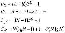
B(K) = (A + K)*2^K + 1; B(0) = A + 1 = 0 --> A = -1; C(2^K) = (K-1)*2^K + 1; C(N) = N*(lg(N) - 1) + 1 = O(N*lg(N))

Merge sorting is thus guaranteed to be of order NlgN for all input data.

Quick Sort

The quick sort algorithm begins by selecting a random element in the array and calling it the pivot. Any element can be used, so the first element is often selected. Then the elements are arranged so that everthing to the left of the pivot has a lower value and everything to the right has a higher value:

Figure showing the array {6,10,19,5,12,0,7,3}. The element 6 is selected as the pivot. After arrangement, the array is {5,0,3, 6 ,10,19,7,12}.

There are several ways to perform this arrange() function. One algorithm is shown in section 7.4.2 of the text and another is in Class 18 on the cs2005 website. The arrange algorithm is linear in the array size N. The quicksort algorithm is recursively called to sort the left and right subarrays. The recursion stops when the array size is one - nothing needs to be sorted. The recurrence relation for the "time" taken by the quicksort algorithm is:

This can represent most of the operations in quicksort, such as comparisions.

The best case is when the pivot always comes out in the middle of the array. Then the two subarrays are equal in size, roughly N/2, and the recurrence relation becomes:

T(N) = T(N/2) + T(N/2) + N; T(N) = 2*T(N/2) = N; T(N) = O(N*lg(N))

The last result comes from noting that the mathematics is the same as the cases of the merge sort, above, and the binary sort, Class 8.

The worst case is when the pivot is always the first or last element in the array. Then one subarray requires no sorting and the other is of size N-1:

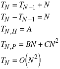
T(N) = T(N-1) + N; T(N) - T(N-1) = N: T(N; homogeneous) = A; T(N; particular) = B*N + C*N^2

Quicksort is normally a fast, efficient algorithm. However, the last calculation shows that quick sort can be a very slow way to sort some special datasets!

To calculate the average time for quicksort - which assumes that the data set contains random values - use the averaging method we introduced in Class 4.

E<T(N)> = sum(all K; Pr{case K} * [T(K; left) + T(K; right) + N]); E<T(N)> = sum(K=1->N; [T(K-1) + T(N-K) + N]) / N; E<T(N)> = N + sum(K=1->N; [T(K-1) + T(N-K)]) / N

In this equation, K represents the location of the pivot in the array and all pivot locations have the same probability: 1/N. This average value can be calculated exactly, as shown on the accompanying page, and it is of the order as the best case: