CS 2223 May 07 2020

Lecture Path: 26
Back Next

Musical Selection: The Ballad of Loki: Songify the Avengers (2019)

Visual Selection: Libro de los juegos (1283)

Daily Question: DAY26 (Problem Set PRABPZKF)

1 Advanced Search Techniques

1.1 Course Errata

Please continue to work on HW4 and the Course Projects.

In class on Monday, I will ask everyone to take some time to complete the survey as well.

1.2 All Pairs Shortest Path

Instead of finding the shortest path from a single source, we often seek the shortest path between any two verices (u, v). There may be several paths with the same total distance. The fastest solution to this problem uses a technique known as Dynamic Programming.

There are two interesting features of dynamic programming:

• It stores the solution to small, constrained versions of the problem

• In addition to finding the optimal answer, you also want to be able to recover the paths themselves. So we need to store additional information to make this happen.

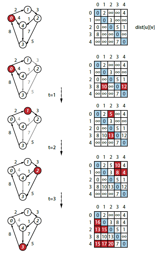
The Floyd-Warshall algorithm computes an n-by-n matrix dist such that for all pairs of vertices, u and v, dist[u][v] contains the length of a shortest path from u to v. The input to the algorithm is a directed, weighted graph G = (V,E). Each edge e=(u,v) has an associated positive weight (i.e., > 0).

It works by computing the dist[][] matrix which represents the shortest distance from each vertex u to every other vertex in the graph (including itself). Note that if dist[u][v] = INFINITY then there is no path from u to v. The actual shortest path between any two vertices can be computed from a second matrix, pred[][], also computed by the algorithm.

// pred[u][v] means "on shortest path from u to v, // last edge came from vertex pred[u][v]." pred = new int[G.V()][G.V()]; dist = new double[G.V()][G.V()]; // initialize edges and base cases for (int u = 0; u < G.V(); u++) { for (int v = 0; v < G.V(); v++) { dist[u][v] = Integer.MAX_VALUE; pred[u][v] = -1; } dist[u][u] = 0; // distance to self is 0 for (DirectedEdge edge : G.adj(u)) { int v = edge.to(); dist[u][v] = edge.weight(); pred[u][v] = u; // base case } } // algorithm now proceeds for (int k = 0; k < G.V(); k++) { for (int u = 0; u < G.V(); u++) { for (int v = 0; v < G.V(); v++) { // can we shorten distance from u to v by going through k. double newLen = dist[u][k] + dist[k][v]; if (newLen < dist[u][v]) { dist[u][v] = newLen; pred[u][v] = pred[k][v]; // TRICK: } } } }

The key insight of this algorithm is the outermost for loop on k.

We make a full sweep through all (u,v) pairs and ask the question: "Can you improve the distance from u to v by trying to go from u to k, and then from k to v?"

As k increases, you eventually try out every possible improvement and ultimately compute the final result. Let’s see this in action:

How would you classify the run-time performance of FloydWarshall? Review the code above and you will see that the primary triply nested for-loop will leads to a classification of O(V3). What about the initialization for-loops? You can see that V2 matrix values are initialized. Then each of the directed edges is visited once in the graph; the initialization is thus O(V2 + E). Altogether, the V3 term dominates, resulting in a total performance classification of O(V3).

Perhaps this isn’t the most efficient solution to the problem. What if we chained together the results of V executions of Dijsktra’s single-source shortest path algorithm? That is, for each vertex, vi execute DijkstraSP(vi). We already know from yesterday that its performance is classified as O((V+E) * log V). So the performance of Chained-Dijkstra-SP – running Dijkstra-SP V times – is O(V * (V+E) * log V).

How do we decide which one to pursue?

Well, for sparse graphs, E is on the order of V (for example, no more than 5*V or some fixed constant). In this case, Chained-Dijkstra-SP would be considered O(V * (V + 5*V) * log V) which is O(V * 6V * log V) and this is O(V2 * log V). This is the clear winner.

However, for dense graphs, E is on the order of V2 (for example, V*(V-1)/4). In this case, Chained-Dijkstra-SP would considered O(V * (V + V*(V-1)/4) * log V) which is O((V*V + V*V*(V-1)/4) * log V) or O(V3 * log V) which would then be outperformed by Floyd Warshall.

I put together a sample program, Compare which demonstrates the side-by-side comparison of these two approaches on random graphs where the number of edges hits the "break-even point". I compute this by considering when:

V3 ~ V*(V+E)*log V.

When E is on the order of V2/log V, you should be able to see that the right-hand side becomes V*V*log V + V*(V*V/log V)*log V which approximates V3. Do not look at these as the equality of two functions – rather, this is where the classification families "overlap".

Here is the output for break-even graphs:

V E time FW time Chained-Dijsktra 16 34 0.0156001 0.0 32 106 0.0 0.0 64 324 0.0 0.0156 128 1107 0.0156 0.0156 256 4077 0.0156 0.0936 512 14705 0.1560 0.1872 1024 52272 1.1232 1.2480 2048 190215 8.5020 10.6860

For dense graphs (i.e., when p = 0.5) the results are noticeably different:

V E time FW time Chained-Dijsktra 16 131 0.0 0.0156 32 517 0.0 0.0 64 2104 0.0 0.0156 128 8121 0.0 0.0624 256 32794 0.0156 0.1560 512 131266 0.1404 1.6692 1024 524532 1.2012 13.7904 2048 2097089 9.4068 123.9583

This completes treatment of graphs. There are many other problems of interest on graphs – many of them are described in the textbook.

1.3 AStar Search Algorithm

We have seen a number of blind searches over graph structures. In their own way, each one stores the active state of the search to make decisions.

• Breadth-First search – Expands the search by refusing to visit vertices n+1 edges away from the start until all vertices n have been searched.

• Depth-First search – Expands the search by randomly choosing a direction, relying on backtracking (via recursion unwinding) to determine alternate routes

• Dijkstra Single-source shortest-path – In searching for the shortest path, Dijkstra makes local decisions to expand the search in the shortest available direction.

These algorithms all make the following assumptions:

• The graph exists in its entirety

• We can identify the vertices in the graph using integers 0 to n-1

• It is possible to mark which vertices have been visited

• There is no way to "know" or "guess" the right direction to proceed

By relaxing these three assumptions we can introduce a different approach entirely that takes advantage of these fundamental mechanics of searching while adding a new twist.

In single-player solitaire games, a player starts from an initial state and makes a number of moves with the intention of reaching a known goal state. We can model this game as a graph, where each vertex represents a state of the game, and an edge exists between two vertices if you can make a move from one state to the other. In many solitaire games, moves are reversible and this would lead to modeling the game using undirected graphs. In some games (i.e., card solitaire), moves cannot be reversed and so these games would be modeled with directed graphs.

Consider the ever-present 8-puzzle in which 8 tiles are placed in a 3x3 grid with one empty space. A tile can be moved into the empty space if it neighbors that space either horizontally or vertically.

The following image demonstrate a sample exploration of the 8-puzzle game from an initial state.

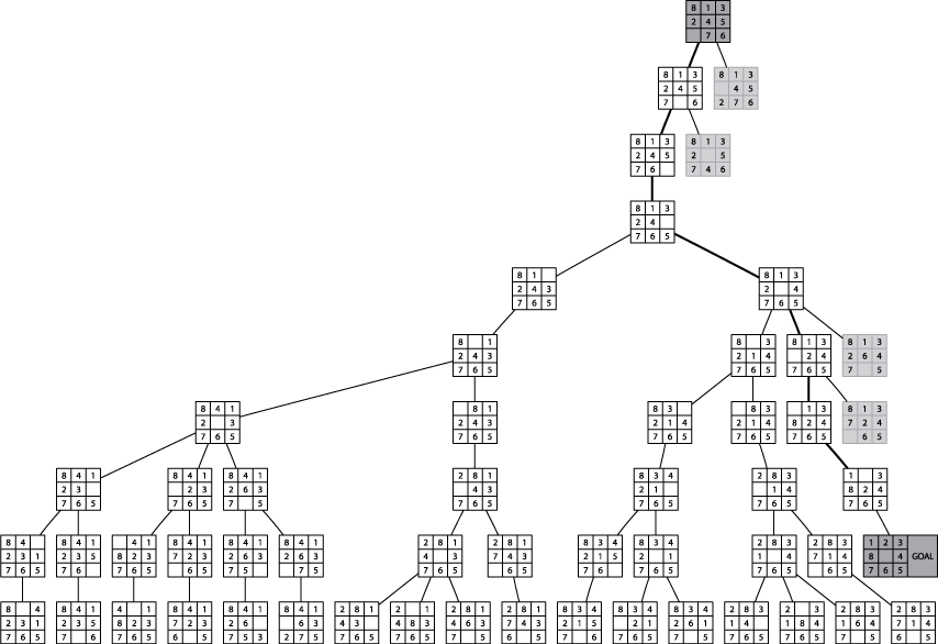
The goal is to achieve a clockwise ordering of tiles with 1 being placed in the upper left corner and the middle square of the grid being empty. Given this graph representation of a game state, how can we design a search algorithm to intelligently search from a starting point to the known goal destination state?

In the field of Artificial Intelligence (AI) this problem is known as Path Finding. The strategy is quite similar to the DFS and BFS searches that we have seen, but you can now take advantage of a special oracle to select the direction that the search will expand.

First start with some preliminary observations:

• The graph is expanded as the search progresses and will never be fully realized.

• Instead of marking vertices, maintain a closed collection of states that have already been visited.

• Make intelligent choices during the search.

In the initial investigations into AI playing games from the 1950s, the following two types are strategies to use:

• Type A: Consider every possible move and select best resulting state based on a scoring function.

• Type B: Use adaptive decisions based upon the knowledge of the game to evaluate the "strength" of intermediate states.

While it is still difficult to develop accurate heuristic scoring functions, this is still an easier task than trying to understand game mechanics.

So we will pursue the development of a heuristic function. To explain how it can be used, consider the following template for a search function:

# states that are still worth exploring; states that are done. open = new collection closed = new collection add start to open while (open is not empty) { select a state n from open for each valid move at that state generate next state if closed contains next { // do something } if open contains next { // do something } else { add next state to open } }

In a Depth-First search of a graph, the open collection can be a stack, and the state removed from open is selected using pop.

The above image shows a max-Depth depth first search which stops searching after a fixed distance. Without this check, it is possible that a DFS will consume vast amounts of resources while darting here and there over a very large graph (on the order of millions of nodes).

In a Breadth-First search of a graph, the open collection is a queue, and the state removed from open is selected using dequeue.

The following represents a BFS on an eight-puzzle search:

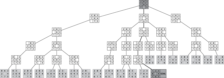
As you can see, this methodically investigates all board states K moves away before investigating states that are K+1 moves away.

Neither blind approach seems useful on real games.

Wouldn’t it be great to remove a state from open that is closest to the goal state? This can be done if we have a heuristic function that estimates the number of moves needed to reach the goal state.

1.4 Heuristic Function

The goal is to evaluate the state of a game and determine how many moves it is from the goal state. This is more of an art form than science, and this represents the real intelligence behind AI-playing games.

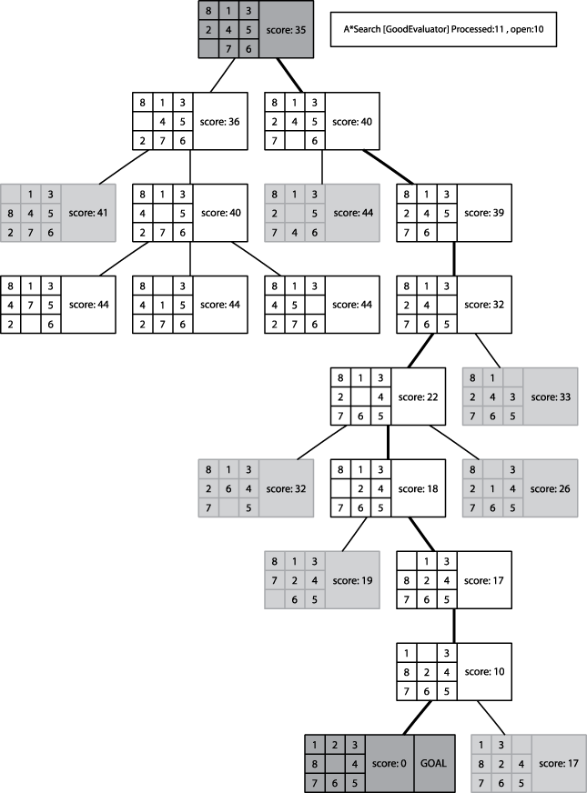
For example, in the 8-puzzle, how can you identify the number of moves from the goal state? You can review the Good Evaluator which makes its determination by counting the number of misplaced tiles while also taking into account the sequence of existing tiles in the board state.

The goal is to compute a number. The smaller the number is, the closer you are to the goal state. Ideally, this function should evaluate to zero when you are on the goal state.

With this in mind, we can now compute a proper evaluation function.

AStar search computes the following function for each board:

f(n) = g(n) + h(n)

Here g(n) is the current depth in the exploration from the start game state while h(n) represents the scoring heuristic function that represents the number of moves until the goal state is reached.

1.4.1 Comparing AStar to BFS

If the Heuristic function always returns 0, then AStar search devolves into BFS, since it will always choose to explore states that are K moves away before investigating states that are K+1 moves away.

It is imperative the the heuristic function doesn’t overestimate the distance to the goal state. If it does, then the AStar search will mistakenly select other states to explore as being more productive.

This concept is captured by the term admissible heuristic function. Such a function never overestimates, though it may underestimate. Naturally, the more accurate the heuristic function, the more productive the search will be.

1.4.2 Sample Behavior

The behavior of AStar is distinctive, as shown below:

1.4.3 Modifying Open States

One thing that is common to both BFS and DFS is that vertices in the graph were marked and they were never considered again. We need a more flexible arrangement. Specifically, if we revisit a state which is currently within the open collection, though it hasn’t yet been selected, it may be the case that a different path (or sequence of moves) has reduced the overall score of g(n) + h(n). For this reason, AStar Search is represented completely using the following algorithm:

public Solution search(EightPuzzleNode initial, EightPuzzleNode goal) { OpenStates open = new OpenStates(); EightPuzzleNode copy = initial.copy(); scoringFunction.score(copy); open.insert(copy); // states we have already visited. SeparateChainingHashST<EightPuzzleNode, EightPuzzleNode> closed; while (!open.isEmpty()) { // Remove node with smallest evaluated score EightPuzzleNode best = open.getMinimum(); // Return if goal state reached. if (best.equals(goal)) { return new Solution (initial, best, true); } closed.put(best,best); // Compute successor states and evaluate for (SlideMove move : best.validMoves()) { EightPuzzleNode successor = best.copy(); move.execute(successor); if (closed.contains(successor)) { continue; } scoringFunction.score(successor); EightPuzzleNode exist = open.contains(successor); if (exist == null || successor.score() < exist.score()) { // remove old one, if it exists, and insert better one if (exist != null) { open.remove(exist); } open.insert(successor); } } } // No solution. return new Solution (initial, goal, false); }

To understand why this code can be efficient, focus on the key operations:

• retrieve state with lowest score in open collection

• add state to closed

• determine if closed contains state

• check if open contains state

• remove state from open

• insert state into open

Clearly we want to use a hash structure to be able to quickly determine if a collection contains an item. This works for the closed state, but not for the open state.

Can you see why?

So we use the following hybrid structure for OpenStates:

public class OpenStates { /** Store all nodes for quick contains check. */ SeparateChainingHashST<EightPuzzleNode, EightPuzzleNode> hash; /** Each node stores a collection of INodes that evaluate to same score. */ AVL<Integer,LinkedList> tree; /** Construct hash to store INode objects. */ public OpenStates () { hash = new SeparateChainingHashST<EightPuzzleNode, EightPuzzleNode>(); tree = new AVL<Integer,LinkedList>(); } }

1.4.4 Demonstration

8 puzzle demonstrations: 8puzzle animations (DFS,BFS,AStarSearch)

Note that it has been shown that every 8-puzzle board state can be solved in 31 moves or less.

Do you find it suprising that with a standard 3x3 rubik’s cube, it has been proved that you can solve any valid random rubik’s cube in 20 moves or less (where any movement of a face counts as a move)? If you prefer the more rigorous quarter-turn metric (where you count each 90-degree rotation of a face as being a move) then the number is 26.

1.4.5 So how good is A* Search

Well, if you try it on larger problems, such as the 15-puzzle, you will find that the search space is too large for most scrambled initial states.

1.5 Interview Challenge

Each Friday I will post a sample interview challenge. During most technical interviews, you will likely be asked to solve a logical problem so the company can see how you think on your feet, and how you defend your answer.

You have a large barrel that stores twelve gallons of water. It is full.

You have an empty seven-gallon barrel and an empty five-gallon barrel.

What sequence of moves must be made to pour exactly six gallons of water into the seven-gallon barrel while leaving exactly six gallons of water in the twelve-gallon barrel?

1.6 Daily Question

The assigned daily question is DAY26 (Problem Set PRABPZKF)

If you have any trouble accessing this question, please let me know immediately on Piazza.

1.7 Version : 2020/05/10

(c) 2020, George Heineman