CS 2223 May 06 2020

Lecture Path: 25
Back Next

Musical Selection: Len: Steal My Sunshine (1999)

Visual Selection: Ancient of Days, William Blake (1757 - 1827)

Daily Question: DAY25 (Problem Set PSABG2FC)

1 Single-Source Shortest Path

1.1 Administrivia

I will remind everyone daily about this course evaluation system.

Next Monday and Tuesday there will be no recorded lectures. Instead, I hope to have a "full Zoom class" on Monday and I would like to encourage as many of you to attend as you can at 10AM. By that date, the course is nearly done, and soon we will be going our separate ways, so I wanted to have at least one "zoom-to-zoom" lecture.

1.2 Variations on SSSP

We now have an algorithm for computing the single-source, shortest path within a weighted, directed graph containing non-negative weights. With the code shown yesterday, the performance is classified as O((V+E) * log V). The book (proposition R on page 654) shortens this to O(E log V) in the worst case. This can be done because E is the dominant value when compared with V.

What if you instead implement the Digraph using an AdjacencyMatrix. What changes with regards to the code, and possibly, the overall performance.

1.3 AdjacencyMatrix representation

An Adjacency matrix representation creates a two-dimensional array which stores the potential edge weights.

public class DigraphAdjacencyMatrix extends EdgeWeightedDigraph{ double[][] weights; public DigraphAdjacencyMatrix (int V) { super(V); weights = new double[V][V]; for (int i = 0; i < V; i++) { for (int j = 0; j < V; j++) { weights[i][j] = Double.NEGATIVE_INFINITY; } } } ... }

We have some choices for specifying "no-edge". One idea is to use an edge weight of "0" for that purpose. Still, we might find ourselves with a graph in which we might allow edge-weights of 0, so we choose to declare a non-existent edge with Double.NEGATIVE_INFINITY.

This representation is unable to determine all adjacent vertices without checking through all possible candidates, thus:

public Iterable<DirectedEdge> adj(int v) { Queue<DirectedEdge> queue = new Queue<DirectedEdge>(); for (int i = 0; i < V; i++) { if (weights[v][i] != Double.NEGATIVE_INFINITY) { queue.enqueue(getEdge(v,i)); } } return queue; }

The reason this becomes a problem for the algorithms we are discussing is that we have been making a common assumption regarding performance of the following code:

for (int u = 0; u < g.V(); u++) { for (int v : g.adj(u)) { statement } }

Earlier this week, I argued that the above code executes statement E times for directed graphs and 2E times for undirected graphs.

Now, however, with an adjacency matrix, the above code will require time that is directly proportional to V2, since the outer u loop executes V times, and each pass through g.adj(u) requires V times as well.

Even worse, the above code is wasteful in that it constructs a queue to contain all edges, when in fact you would do better to optimize the DijkstraSP code to work directly off of a 2D array.

N #Edges Time-List Time-Matrix 128 3246 0.000000 0.000000 256 13091 0.000000 0.000000 512 52209 0.000000 0.016000 1024 209471 0.015000 0.000000 2048 838639 0.000000 0.047000 4096 3354546 0.031000 0.171000 8192 13421744 0.156000 3.229000

Using the small example code CompareDensePerformance, the performance is 20x slower with matrix representation.

1.4 Variations on Single-Source Shortest Path

There are several variations that might be considered (p. 654).

1.4.1 Undirected graphs

1.4.2 Directed Acyclic Graphs

What if you know the graph is a DAG, that is, there are no cycles? A more efficient variation of Dijkstra’s SP algorithm (page 658) is to relax the vertices in topological sort order. Since you know there are no cycles, each edge is going to be visited exactly once. This approach doesn’t need to use a priority queue, which means its performance is based on the performance of Topological Sort (p. 583) which means the worst case is O(E + V). This is a noticeable improvement over O(E*log V).

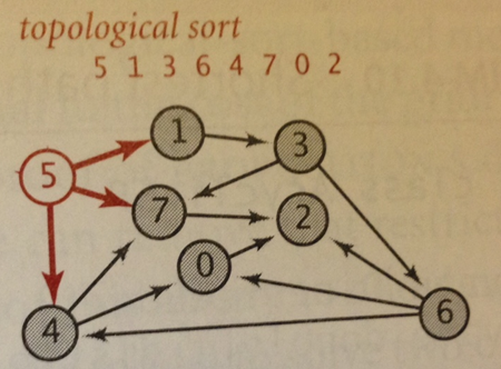
Here is a sketch of the algorithm. Once the topological order is computed, you process each vertex in order, relaxing all edges from those vertices. Note there is no need to use a priority queue because you rely on the topological sort to give you the vertices in a proper order; certainly, you might find a better shortest path with more edges, which forces a relax operation, but this won’t affect the order in which you process the vertices.

// Relax without a priority queue since Acyclic void relax (EdgeWeightedGraph G, int v) { for (DirectedEdge e : G.adj(v) { int w = e.to(); if (dist[w] > dist[v] + e.weight()) { distTo[w] = dist[v] + e.weight(); edgeTo[w] = e; } } } void shortestPath(EdgeWeightedGraph G, int s) { Topological top = new Topological(G); // Process each vertex in order for (int v : top.order()) { relax (G,v); } }

1.4.3 Negative Edge Weights

What if we wanted to allow edge weights to be negative. This fundamentally alters the nature of the problem.

Note that Dijkstra’s SP algorithm used a priority queue to determine the order of vertices to investigate. And the claim was that the vertices removed from the priority queue were done in shortest distance from the source. This claim was made possible because successive paths only increased the total distance, so now our original assumption is invalid.

Consider the following small graph:

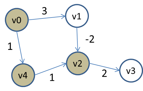
The vertices are colored based on whether they have been processed and removed from the priority queue. As usual, we compute Single-Source Shortest path starting from vertex v0. All vertices in the priority queue have INFINITY as distance (except for v0 which is the source). After removing v0, it updates the distances for v1 and v4 because of the existing edges to those vertices. Now, v4 is the first to be removed, since its total distance is 1, placing it at the "top" of the priority queue, which vertex v1 has distance of 3, placing it second. Once v4 is removed, the edge to v2 relaxes that distance.

Thus vertex v2 is adjusted (that is, decreaseKey is called) and the priority queue contains three vertices with the following distance (aka, priorities):

• v2 with distance 2

• v1 with distance 3

• v3 with distance INFINITY

Naturally, it removes v2 from the priority queue and eventually v3 is adjusted with a total distance/priority of 4.

As you can see, Dijsktra’s SP algorithm just "assumes" that any edge coming from v1 to v2 will only increase the total accumulated weight, however, when removing v1 from the priority queue (since it is the lowest distance), it suddenly sees an opportunity to reduce the total distance to v2.

However v2 has been removed from the priority queue and so it can’t be relaxed. In fact, if you try to do this, the code will throw an exception. You could choose to "mask" this exceptional case, by modifying the DijkstraSP code as follows:

void relax(DirectedEdge e) { int v = e.from(); int w = e.to(); // distance from s ->v + edge weight (v, w) < distance from s to w if (distTo[w] > distTo[v] + e.weight()) { distTo[w] = distTo[v] + e.weight(); edgeTo[w] = e; if (pq.contains(w)) { pq.decreaseKey(w, distTo[w]); } } }

And this would work for a little while... but it won’t last.

There is one more awkward situation to deal with. What if there is a negative cycle, that is, a directed cycle whose total weight (sum of the weights of the edges) is negative. If such a cycle existed, one could arbitrarily lower the total path cost by simply iterating through thus cycle as many times as you would like. So we must find a way to detect negative cycles in any graph that allows negative weights.

1.5 Bellman-Ford Algorithm

The book describes Bellman-Ford in a way that is more complicated than it needs to be. Bellman-Ford has the same approach that Dijkstra’s has, namely, find some edge to relax (or lower) distance. However, instead of trying to find vertices from which we relax individual edges, Bellman-Ford processes all edges within a fixed number of iterations.

int n = G.V(); for (int i = 1; i <= n; i++) { // for each edge in the graph, see if we can relax for (DirectedEdge e : G.edges()) { if (relax(e)) { if (i == n) { return; // negative cycle. DONE } } } }

And here is the relaxation code, as expected. For convenience, it returns true if the edge reduces the best shortest path.

boolean relax(DirectedEdge e) { int v = e.from(); int w = e.to(); if (distTo[w] > distTo[v] + e.weight()) { distTo[w] = distTo[v] + e.weight(); edgeTo[w] = e; return true; } return false; }

The best part of Bellman-Ford is that you don’t need to check for negative cycles. In each iteration (there are N of them where N=V) you process all edges to see if you can relax the distance. If you make a full pass over all the edges and you did not find a single edge to relax, then you know that you are done.

Let’s analyze the performance of this code. The outer for loop executes V time, and the inner for loop executes E times, thus the performance of this code is Θ(E*V).

However, what if you keep making iterations, and keep finding edges that seem to relax a distance, here and there. How do you know if you are still making progress to the actual solution? It turns out there is a very simple answer to this question.

I’ll start by asking this: What is the longest possible path between any two vertices in a directed weighted graph? Well, if there are V vertices, then it must be V-1 edges.

So, thinking along the lines of breadth first search, if you start at a source and complete one iteration over all edges, you know that you have the shortest distance between source and all vertices one edge away. After the second iteration, you know that you have the shortest distance between source all all vertices two (or fewer) edges away. If you continue through V-1 iterations, you will have completed the solution.

However, what if a negative cycle exists? Well, then go ahead and iterate one more time, and if you find an edge that relaxes a distance value, you know there must be a negative cycle.

This is why the for loop iterates exactly V times.

There is also a nice optimization here. It may turn out that after a few iterations, you find no other edge that can be relaxed. In this case, perhaps long before V, you can stop and declare a solution.

If you look at the code, you will see how we handle these two edge cases.

1.6 Big Theta Notation

Can you explain why "T(n) = N - 999" is classified as Θ(N).

Try to find c1 such that for all N > n0, c1*N < N - 999.

Now try to find c2 such that for all N > n0, c2*N > N - 999.

If you can find these three constants (c1, c2 and n0) then you can claim that T(n) is Θ(N).

1.7 Daily Question

The assigned daily question is DAY25 (Problem Set PSABG2FC)

If you have any trouble accessing this question, please let me know immediately on Piazza.

1.8 Version : 2020/05/10

(c) 2020, George Heineman