The transform process can be thought of as decomposing an image into a sequence of basis images - taking the transform is simply the process of calculating the constant to multiply each of the basis images by before summing them to produce the image. That understanding can be used to develop an intuition about the appearance of the transform image.
We also talked about multiplicative constants in transforms and how Parseval's theorem
![]()
can be used to decide where to use the constants. It also provides an important check on transform algorithms.
Much of the value of using Fourier transforms comes from understanding its properties and how to use them. Many of these properties are summarized in Tables 2.3 of the text.
For example, a spatial shift in an image produces a frequency-dependent phase shift in the transform.
![]()
Recall that the transform of the rectangle or sampling function is the sync function, as shown in Class 4, The sync function is real so the transform of a rectangle centered at the origin is real. If it is shifted away from the origin, the frequency-dependent phase shift makes the transform complex at some frequecies;
![]()
Conversely, if the transform is shifted in frequency space, there will be a resulting position-dependent phase shift in the image. But, images cannot be complex; gray levels or colors values are always real and positive. Thus all images have transforms that are symmetric about the axis in frequency space. In particular, every function (including images) can be expressed as the sum of even and odd parts. This symmetry carries over into the transforms:
| function f(x) | transformF(u) |
| even | even |
| odd | odd |
| real and even | real and even |
| real and odd | imaginary and odd |
We'll prove the first property to give you the flavor of how it is done.
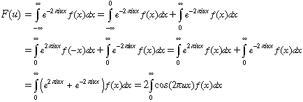
If f(x) is even, then f(-x) = f(x). Look at its transform:

The first step is to split the integral into two parts. Then the order of integration is switched in the first integral by replacing x by -x and the evenness of f(x) is used explitly to eliminate f(-x). The two itegrals are combined using the linearity of the integration function and the Euler equation is used to replace the exponentials by the cos() function. Since cos() is an even function, and since u appears only in the cos(), F(u) must be even: F(-u) = F(u).
Look in detail at what happens to the even and odd parts of a function,
![]()
The properties table shows that Fe(u) and Fo(u) are real. Then the magnitude and phase of F(u) are:

Thus, the magnitude of the transform of any real image is even and the phase is odd. This can easily be seen, for example, in the Solution in Homework 3. An understanding of symmetry in transforms can often lead to a significant improvement in execution times of transform algorithms.
Here are three references about the Hartley Transform
The key points that make the Hartley transform useful are:
These are point transforms, which turn one gray level (or color) into another. These transformations are usually implement by means of a lookup table (input values are byte offsets from the beginning of an array of bytes, which represent the output values) .
As an example of a point transform, consider the problem of stretching/compressing
pixel values so that the min and max values map into the extrem pixel values
(usually 0 and 255). Assume WHITE and BLACK are
the extreme pixel values and min and max are,
respectively, the lowest and highest pixel values in an image (which can
be bytes, integers, floats, doubles, etc.). WHITE and BLACK
are shown in all caps because they are usually defined as macros in image
processing code.
The most general linear equation for determining a new gray level value is:
![]()
If, for example, we assign WHITE to min and
BLACK to max, we can solve for values for A
and B.

This gives the final transformation equation:
![]()
Of course, it will be necessary to assure that g never falls outside
the range (min, max) and to be sure that min
and max are never equal!
Non-linear operators can be used, too. The log operation is particularly useful for enhancing images with great range in pixel values (such as transform magnitude images). However, be sure that you don't try to take the log of a negative number or zero. It is worth thinking about how to achieve this.
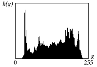
A histogram h(g) is a function that counts the number of pixels at some gray level g.

For a number of reasons, including the "spikiness" (this is not necessarily a continuous function), the integral of this function is often used. Here is a simplified example.

This function, ![]() , is called the cumulative probability distribution
function and its derivative, p(g), is the probability density function,
roughly the probability that a pixel has the graylevel g.
, is called the cumulative probability distribution
function and its derivative, p(g), is the probability density function,
roughly the probability that a pixel has the graylevel g.


The notation n has been used inside the summations, but it's really just a graylevel g.
In general, any point transformation - such as the linear transformation shown above - can be written as a function of g:
![]()
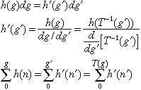
If we assume T(g) is continuous, the pixels with gray levels between g and dg in the original image map into a similar gray-level region in the final image: This equality results in two equivalent expressions relating the two histograms (before and after point transformation), one differential and one integral (summation):

So far, this analysis is general; it is made much easier if T is invertable, but that is usually difficult. Thus the summation form is used.
A useful image enhancement technique is histogram equalization. That means that we want to select a transformation T which results in a "flat" histogram; p(g) is the same for all values of g. Restaate the last equation in terms of probabilities:

The leading factors have been eliminated because they equal the same thing - the number of pixels in the image.If the new histogram is to be flat, we can replace the probability on the right side by a constant and take it outside the summation:
![]()
The transfer function is proportional to the cumulative distribution function. The constant is selected to make sure that the value of T(255) is 255. If a pixel's old value was g then the new value is the maximum gray level (255) times the fraction of pixels with gray levels g and below:

Note that the denominator is just N, the number of pixels in the image.