Forward and Inverse Fourier Transforms
The Fourier transforms of a function is an integral of the form
![]()
and its inverse function is
![]()
The exponential kernel is what makes it a Fourier transform -
other integral transformations have other kernels. Two subjects of great
religious debate among applied mathematician is where, precisely, to put
the ![]() and whether to use i or j to represent
and whether to use i or j to represent ![]() .
.
The Fourier Transform of a Constant
The Fourier transform of a constant is a delta function. Here is how to demonstrate that:
Straighforward way
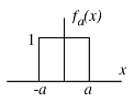
What is the Fourier transform ![]() which corresponds to the function
which corresponds to the function
![]()
Try plugging that function into the Fourier transform:
![]()
This integral doesn't converge so we need to use....
A Mathematical Trick
Consider a sequence of functions such that:
![]()
where
![]()
We use this to calculate the corresponding Fourier transform
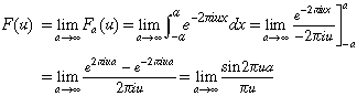
Unfortunately, this equation doesn't converge, either.
The problem is that our ![]() is too sharp. All of its derivatives (first,
second, ...) are infinite. So, let's try...
is too sharp. All of its derivatives (first,
second, ...) are infinite. So, let's try...
Yet Another Mathematical Trick
Try a function wich is "smoother", which means its derivatives fall off with repeated differentiation.
![]()
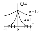
As a goes to infinity, the exponent goes to zero so the function becomes the constant we are seeking. Calculate the Fourier transform:
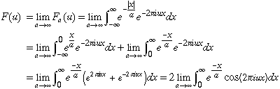
We can evaluate the integral by using the following result, which is equation 4.3.137 in Abramowitz and Stegun,
![]()
The Fourier transform is:
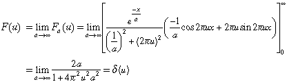
The last step is not obvious, so we will test that the answer obeys the three properties of the delta function:
![]()
Using L'Hopital's rule, we can evaluate the limit:
![]()
This satisfies two of the three properties of the delta function since the limit as a increases is infinity or zero depending on whether or not u is zero. To test the third property, we need to evaluate the integral
![]()
Equation 3.3.21 in Abramowitz and Stegun is:
![]()
So we can evaluate the integral to get:
![]()
This demonstrates that the Fourier transform of a constant is an impulse (and vice-versa).
What does this all mean?
We chose this example because it illustrates several things.
First, the actualy process of finding a Fourier transform of a function in closed form is a specialized mathematical process that only works for some functions and is rarely straightforward. That is why people who use Fourier transforms put considerable effort into modeling signals (images, in our case) using functions whose transforms have already been evaluated by others.
Second, there is no reason to be frightened by delta functions. They are a convenient way to model sampling at a single point in space or frequency. When you acatually do anything with transforms, the delta functions get integrated away. If you ever end up with a delta function in the signal representing an image, you've done something wrong. Delta functions in transforms are ok, just not in images. In fact, we now know that the Fourier transform of a featureless, uniformly-gray image is just a single non-zero value in the Fourier transform.
Finally, recall the point made several times in class. The real value in understanding transform theory is not in being able to find transforms of some functions, but in understanding the properties of transforms, including those in Table 4.1 in the text.
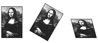
Here is one more example of how to work with Fourier transforms. The affine transformation is a class of geometric transformations that is useful in image processing. For example, these are the same image, but the second is rotated and the third is squashed and sheared.
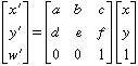
In all of these cases, the transformation can be described by noting where the graylevel at the pixel (x,y) ends up after the transformation. In affine transformations, this can be described by 6 numbers:
![]()
This is just matrix notation for two linear equations:
![]()
In computer graphics, the equations are often expressed in the form of homogeneous coordinates
where w is an extra coordinate whose value is divided into the others to calcualte the actual spatial coordinates. If the analysis is extended into 3D, affine transformations can be used to represent a wider range of geometric distortions, such as the perspetive projection found in photographic images taken using a tilted camera.
Note: if you are interested, material on affine transformations is covered in WPI courses CS 4731 and CS 543.
The question is this: if the Fourier transform of an image is known before affine transformation, how can it be used to calculate the Fourier transform of the image after affine transformation? In other words, if we know the image and its Fourier transform:
![]()
and if we know the affine transformation that alters the image,
![]()
how can we calculate the transform of the affine transformed image?
![]()
The generic form of the 2D Fourier tranform is:
![]()
Unfortunately, we can't just plug in the transformed function
![]()
because the integral can't be evaluated - it contains all four x
and y variables, ![]() . Since the function
. Since the function ![]() is in the transformed
variables, let's try to eliminate the x and y from the integral
so that it can be solved. Specifically, try to get it in this form:
is in the transformed
variables, let's try to eliminate the x and y from the integral
so that it can be solved. Specifically, try to get it in this form:
![]()
The equations for the transformed variables can be inverted:
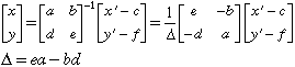
This inversion method only works for 2x2 matrices and fails when the determinant is non-zero (the matrix is singular). Begin by calculating the differentials:
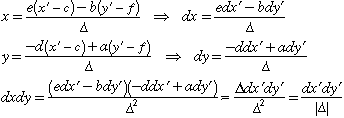
The approximation is justified because squares of differentials can be eliminated from integrals.
Next substitute variables in the exponential
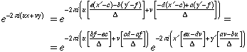
The first factor is a contstant (it doesn't contain x' or y') and the second is in the form shown above. Combining these results, we obtain:
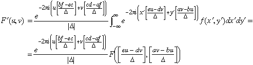
So What?
Apart from being useful in its own right, this result can be used to calcualte/verify other results.
Image Shift
Consider the case where an image is shifted to the right. This corresponds to the affine transformation:
![]()
and our general equation reduces to:
![]()
which is the result shown in Table 4.1 of the text. From the form of the general affine equation, we see that the constant in front is always one unless there is a shift in some direction.
Image Rotation
Assume that the image is rotated through the angle![]() (counter-clockwise
is positive). Then the matrix elements and transform become:
(counter-clockwise
is positive). Then the matrix elements and transform become:
![]()
Other results which follow directly from the affine transformation equation are Linearity and Scaling.