 T1 := A + A
OPT.0 Introduction
This chapter uses the material of the last two chapters to describe program improvements. We divide optimizations into three categories: (i) local optimizations, (ii) global optimizations and (iii) loop optimizations. Chapter 11 discusses another way to improve programs by allocating registers creatively. The last program improvement, peephole optimization, which is performed after code is selected, is also discussed in Chapter 11.
We also include two examples, one which optimizes on the control flow graph and one which optimizes at a higher level on the abstract syntax tree.
We show much of the intermediate representation in this chapter as quadruples; they are much easier to read than abstract syntax trees. This method suffers from the Heisenberg Uncertainty Principle (which the reader may remember from chemistry or physics); it affects the very code we are trying to improve. Quadruples introduce many temporary variables which we will eliminate when possible. Otherwise, the same information can be discovered in trees as in three-address code. Throughout this chapter, we use the term optimization, knowing that we really mean improvement.
Local optimizations improve code within basic blocks. Although the separation is somewhat hazy, we won't include as a local optimization anything that moves code outside a block or uses information from outside a block.
In a sense, this category is redundant. Almost all local optimizations have their global counterpart. The method of detection is often different, however.
EXAMPLE 2 Local common subexpression elimination
 T1 := A + A
Constants are produced, not only by the programmer, but also by the compiler. The programmer may initialize a variable to be 1, using this as both the loop counter and as an array index. Then, in allocating space for the array, the compiler may multiply such elements by 4 to indicate that they are to use four bytes of storage.
EXAMPLE 3 Local constant propagation
I := 2 I := 2
...  ...
...
T1 := 4 * I T1 := 4 * 2
A related optimization computes constant expressions at compile-time rather than generating code to perform the optimization.
EXAMPLE 4 Local constant folding
I := 2 I := 2
...  ...
...
T1 := 4 * I T1 := 8
Constant folding is sometimes called constant computation.
It can require a little more alertness on the part of the compiler, as
shown in Example 5.
EXAMPLE 5 Local constant folding
    I := 2 * I

  I := 8 * I

    (no reference to I)

    I := 4 * I
Here, I has been modified twice.
An algebraic identity performs a substitution using algebraic laws. We list a few:
1. X := A + 0X := A 2. X := 1 * A
X := A 3. Constant * Symbol
Symbol * Constant
Algebraic substitution can substitute one expression in a basic block with another as shown in Example 6.
EXAMPLE 6 Algebraic Substitution
          T1 := BB * J - 1           T1 := BB * J - 1

          ...                     ...

          T1 := T1 + 1               T7 := 4 * J
Most programs spend the majority of their time in loops. The payoff in optimizing loops is, on the average, greater than any other optimization.
In Module 7, we discussed how to identify a loop. We use that here when performing loop optimizations.
In particular, there is a useful property of loops: two natural loops are either disjoint (except for the header) or one is nested within the other.
Two loops with the same header should probably be merged into one:

We will use the property that two natural loops are either nested or disjoint for some loop optimizations. The two most common optimizations are detection and movement of invariant code and induction variable elimination. Other optimizations optimize special loop forms such as loops which make changes to array elements one by one or pairs of loops with the same execution conditions.
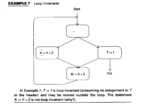
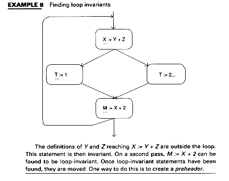
Loop-invariant statements are shose statements within a loop which produce the same value each time the loop is executed. We identify them and then move them outside the loop.
Example 7 shows a control flow graph and a loop-invariant statement.
Preheaders
For each loop, create a new block, which has only the header as a successor. This is called a preheader and is not part of the loop. It is used to hold statements moved out of the loop. Here, these are the loop-invariant statements. In the next section, the preheader will be used to hold initializations for the induction variables.
Code Motion Algorithm
If a statements is loop-invariant, it is moved to the preheader provided (1) the movement does not change what the program computes and 2) the program does not slow up.
Algorithm
Loop-Invariant Code Motion
Given the nodes in a loop, compute the definitions reaching the header
and dominator.
Find the loop-invariant statements.
Find the exits of the loop: the nodes with a successor outside the loop.
Select for code motion those statements that:
(i) are loop-invariant and
(ii) are in blocks that dominate exits and
(iii) are in blocks that dominate all blocks in the loop which use their
computed values and
(iv) assign to variables not assigned to elsewhere in loop
Perform a depth-first search of the loop. Visit each block in depth-first order, moving all statements selected above to the preheader.
The last step preserves the execution order.
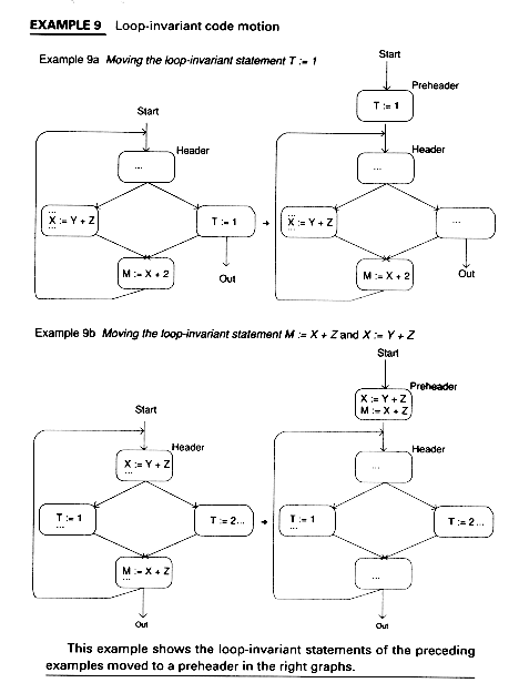
Moving statements to the preheader may cause the program to slow down if the loop is never entered. The criterion that the loop never slow down may be enforced by executing the statements in the preheader only if the loop is executed.
Taking this one step further, the condition:
WHILE Condition DO Statements
becomes
IF Condition
Now the preheader is executed only if the loop is entered.
An induction variable is a variable whose value on each loop iteration is a linear function of the iteration index. When such variables and the expressions they compute are found, often the variable itself can be eliminated or a strength reduction can be performed.
EXAMPLE 10 Induction variable
J := 0
FOR I := 1 to N DO
J, K and M are all induction variables. (The loop index, i, is trivally an induction variable.)
EXAMPLE 11 More induction variables
t := b * c
FOR i := 1 TO10000 DO
...
...
d is an induction variable.
The most common induction variables are those which result from indexing elements of an array. Multiplications of the index are created when an array takes more than one byte or when the offset is computed for multidimensional array.
Induction Variables
We find induction variables incrementally. A basic induction variable is a variable X whose only assignments within the loop are of the form:
X := X + C
X := X - C
where C is a constant or a loop-invariant variable. In Example 10, I and J are basic induction variables.
We define an induction variable, recursively, to be a basic induction variable or one which is linear function of some induction variable. In Example 10, K is an induction variable since K is a linear function of J. M is an induction variable since M := 3 * K = 3 * (2 * J) = 6 * J. The expressions J + 1, 2 * J, and 3 * K are called induction expressions.
Finding Induction Variables
After reaching definitions find all definitions of Y and Z in X := Y op Z which reach the beginning of the loop, basic induction variables can be found by a simple scan of the loop. To find other induction variables, we find variables, W , such that
W := A * X + B
where A and B are constants or loop invariants, and X is an induction variable. These can be found by iterating through the loop until no more induction variables are found.
In Example 10, the variable J reaches the top of the loop. The statement J := J + 1 satisfies the definition of a basic induction variable. The other statements will be found on successive visits through the loop.
Although strength reduction is, strictly speaking, a global optimization, it rarely pays off except in loops.
Consider the multiplication in Example 11. Since d is an induction variable, we can replace the induction expression i * 3 by initializing d to its initial value, 3, outside the loop and then adding 3 on each loop iteration. This is shown in Example 12.
EXAMPLE 12 Strength reduction
        t := b * c                      t := b * c

         FOR i := 1 to 10000 DO          d := 0

          BEGIN                          FOR i := 1 TO 10000 DO

            a := t                       BEGIN

            d := i * 3                           a := t

            ...                                  d := d + 3

          END                                    ...

                                           END
We have shown the example for a strength reduction of a multiplication to an addition, but other strength reductions may be performed also (see Exercise 7).
We list some other optimizations for loops here, with the exercises exploring how these optimizations would be found from data flow analyses, loop invariants and loop inductions.
Loop unrolling decreases the number of iterations of a loop. Consider the following loop:
LOOP I = 1 to 10000 by 1
ENDLOOP
Unrolling by 2 gives
LOOP I = 1 to 9999 by 2
The number of instructions executed is reduced because the number of increments and tests is halved.
Another example of loop unrolling is:
      WHILE Condition                  WHILE Condition

          A                              A

       ENDWHILE                           IF NOT Condition THEN Exit

                                             A

                                        ENDLOOP
A
ENDWHILE IF NOT Condition THEN Exit
A
ENDLOOP
Loop unrolling also exposes instructions for parallel execution since the two statements can be executed at the same time if they are independent
The disadvantage here is that increased instruction space is required.
Sometimes two loops may be replaced by one. Consider the following loops:
LOOP I = 1 to 100
These two loops can be "fused":
LOOP I = 1 to 100
The loop overhead is reduced, resulting in a speed-up in execution, as well as a reduction in code space. Once again, instructions are exposed for parallel execution.
The conditions for performing this optimization are that the loop indices be the same, and the computations in one loop cannot depend on the computations in the other loop.
Sometimes loops may be fused when one loop index is a subset of the other:
FOR I := 1 TO10000 DO
FOR J := 1 TO 5000 DO

FOR I := 1 to 10000 DO
This transformation simplifies the termination test (computers often have separate instructions to test for 0):
     LOOP FOR I := 1 TO N DO         LOOP FOR I := 1 - N TO 0


            ...I...                         ...I + N...


      ENDLOOP                         ENDLOOP
LOOP FOR I := 1 TO 1000
IF (Test) THEN
Here, the test is performed each time through the loop. The following performs the test once:
IF (Test) THEN
The second version here reduces the number of instructions executed,
but the code takes more space.
Sometimes, as the result of other optimizations, the body of a loop becomes vacuous. It may then be removed:
    LOOP

     ENDLOOP              Null
Null
Many global optimizations are analogous to local ones, but use data flow analysis to find optimizations between blocks. Even though we include them here, in global optimization, their payoff is greater when they also reduce the computations in a loop.
Figure 1 shows an expression X op Y which may be computed once on each path and then used.
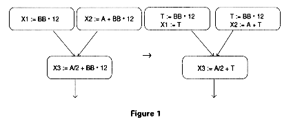
From reaching definitions, a use-definition chain, ud-chain, can be constructed. This is a list of variable definitions linked with their uses. Within a block, a definition is matched to its subsequent use. If there is no definition within the block, then all definitions which reach the block are matched with the use.
The ud-chain may be used for constant propagation.
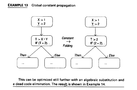
This can be optimized still further with an algebraic substitution and a dead code elimination. The result is shown in Example 14.

As the result of previous optimizations, both statements and entire blocks may now be unnecessary.
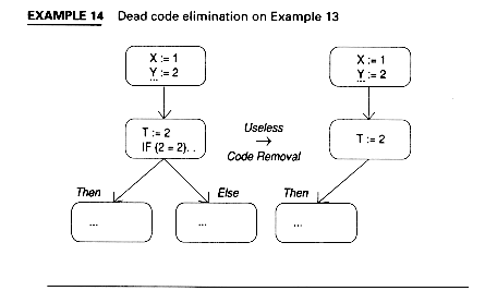
The general cases for Example 14 are:
IF True THEN AA ELSE B
and
IF False THEN AB ELSE B
Sometimes a conditional can be reordered:
IF Condition THEN IF NOT Condition THEN NullA ELSE A ENDIF ENDIF
If it is known via data flow analysis and perhaps other optimizations that Value(A) = Value(B), then
A := BNull
This presumes that A and B really are the same variable; that is, they are not both needed later.
The following code is often generated by IF-THEN_ELSE statements or CASE statements:
GOTO LabelA GOTO LabelB ...... LabelA: GOTO LabelB LabelA: GOTO LabelB
This presumes that A and B really are the same variable; that is, they are not both needed later.
Computing the offsets for array references is time consuming and may often be eliminated when the value is used:
A[I,J] := B * C T := B * C ...... A[J,I] := A[I,J] + 1 A[J,I] := T + 1
This presumes that A and B really are the same variable; that is, they are not both needed later.
In this section, we perform an example which includes many of the optimizations discussed so far:
Consider the algorithm for a Bubblesort from Chapter 7:
 FOR I := 1 TO N - 1 DO

   FOR J := 1 TO i DO

     IF A[J]  > A[J + 1] THEN

       Temp := A[J]

       A[J] := A[J + 1]

     ENDIF

   ENDFOR

 ENDFOR
The intermediate representation (shown as quadruples) and the control flow graph are:
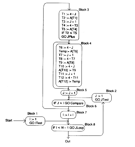
One of the best optimizations here would be an algorithm optimization, which would replace Bubblesort with a better algorithm such as Quicksort. We won't do this however.
There are algebraic optimizations here: T4 computes 4 * T3 = 4 * (J + 1) = 4 * J + 4. Similarly, T8 computes 4 * T7 = 4 * ( J + 1) = 4 * J + 4 and T12 = 4 * T11 = 4 * (J + 1) = 4 * J + 4. Changing these:
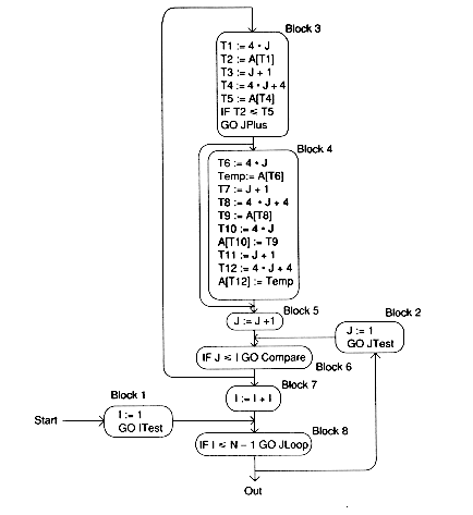
We look for some local optimizations which can be performed within the basic blocks.
There is local common subexpression elimination to be performed in our example. In Block 3, both T1 and T4 compute 4 * J. In Block 4, T6, T8, T10, and T12 compute 4 * J; both T7 and T11 compute J + 1; both T8 and T12 compute 4 * J + 4.
We will replace the second occurrence of 4 * J in Block 3 by its value, T1, and the second, third and fourth occurrence in Block 4 by the computed value T6, T3, T7, and T11 go away:
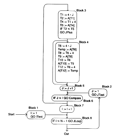
There is no opportunity for local constant folding or elimination unless n is known at compile time.
We move on to global and loop optimizations, presuming that data flow analysis has been performed (see Module 9, Exercise 2).
In Block 4, A[T6] which is A[4*J] is computed in Block 3. Control flow analysis tells us that we can't get to Block 4 without going through Block 3, and data flow analysis tells us that J doesn't change in between. Thus, we replace the first two statements in Block 4 by:
Temp := T2
Similarly, T10 is the same as T1, T8 is the same as T4, and T12 is the same as T4.
Block 4 becomes:
Temp := T1 A[T1] := T5 A[T1] := T5A[T4] := T1 A[T4] := Temp
Looking at the revised program:
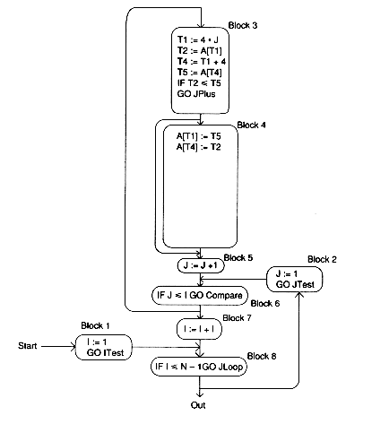
Next, we find the natural loops in order to perform induction-variable elimination. It is somewhat difficult to find the header of the inner loop because of the way the control flow graph is drawn, but Block 6 satisfies the definition from Module 7 (the reader is invited to check this). The loops are {6,3,4,5} and {2,3,4,5,6,7,8}.
For the loop, {Block 6, Block 3, Block 4, Block 5}, there are induction variables J (incremented by 1) and T1 and T4 (incremented by 4)
In Block 3:
 T1 = 4 * J

 T4 = 4 * J + 4
We can eliminate J, replacing the test on J with one on T1:
IF J<= IIF T1 <= 4 * I
Note that J cannot be eliminated if it is to be used later in the program.
The new Block 6 becomes:
 T14 := 4 * I

 IF T1 <= T14 GO JLoop
In Block2, we eliminate the initialization of J and replace it with a new Block 2:
Block 2 is functining as a preheader here. We also need to replace the increment of J by an increment of T1 and T4. The new code is:
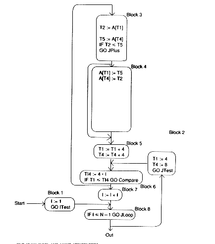
We new look for loop invariants .
T14 := 4 * I
is invariant in the inner loop, and we move it to Block 2:
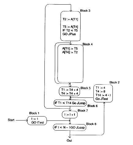
The final code is much improved over that shown originally. The reader is invited to search for more optimization to be performed here.
Loveman(1977) describes the optimization phase as the "term given to the application of a set of rules for manipulating various representations of a program by exploiting local or global invariances within the program in order to improve the program relative to some measure."
In what follows, we assume a tree-structured representation and that the optimizations shown are really parttern-directed rearrangements of program text. As before, it is easier for humans to see this in source form or as quadruples.
The transformations are not applied in a random order; the successful appliction of one transformation suggests successor transformations. In fact, transformation ordering and information gathering is a major part of this method.
In addition, some transformations may not improve the program, but may lead to other transformations which do optimized. Similarly, some transformations may be machine-independent, but the reason for applying one may depend on the target machine.
This chapter has discussed a large number of optimizations, most of which are found on the control flow graph. The reader may be wondering what the improvements really are. Is it worth the time and effort at compile time -- not to mention at compiler creation time -- to perform such aggressive optimizations?
The answer is -- it depends. Statistics have shown that there is a 5-25% improvement in running time for the loop optimizations:
There is a 1-5% improvement for:
Interestingly, the topic of the next chapter, register allocation, has been shown to improve code more than the optimizations above. Because good register alloction does improve code, it is often discussed in chapters on optimization.
The optimizations performed after code generation, peephole optimization, also have a high payoff. We discuss these in Chapter 11.
Procedure calls may be approached in two ways. The first is to assume the worst case for the call, and the second is to actually perform the data flow analyses throughout the procedure.
For the first approach, default assumptions include assuming no definitions are killed, expressions are nolonger available, etc.
Approach two requires careful following of aliases. An alias is another name for a location. REference parameters are aliases for the actual arguments. Once aliases are identified, the analysis is similar to intraprocedural analysis.
This chapter has used the results of the last two chapters to improve programs so that the ultimate code executes faster. In some cases, this also performs a space improvement; in some cases the improvement in time produces code which consumes more space.
We divide these improvements into three catagories: local, loop and global. The divisions are somewhat arbitrary in that loop optimizations may be classified as either local or global. Loop optimizations, in general, improve code more that other optimizations.
There are two more improvements, often categorized as optimizations because they improve program performance greatly: good register allocation and peephole optimization