CS 2223 Apr 13 2023
Expected reading:
Visual Selection: Still Life, Severin Rossen (1849)
Live Selection: Creep by Radiohead, cover Thalia Strings (2015)
Jazz Selection: Keith Jarrett ~ Expectations (1969)
1 BST recursions and Asymptotic Notation
I am going to finish describing recursive methods within BSTs. We will also more formally present Big O notation and explain it mathematically.
But first, insert the following keys into a BST and we will discuss the final result...
N, E, S, I, O, C, R, Y, D, B, A
1.1 Computing Floor(key) in BST
This section was introduced on day 15 but I didn’t cover it in class. You can cover this in more detail on your own.
Let’s tackle a more challenging question. How about returning the keys in a BST that are closest to a target key, without actually being present in the BST? We use the mathematical concept of Floor and Ceiling as follows:
Floor – find the largest key that is smaller than target
Ceiling – find the smallest key that is larger than target
In a way, you have seen this concept in Binary Array Search. Try the following example by hand:
Search for the value 7 in a sorted array:
+—
When Binary Array Search completes without finding a value, note that the value of lo points to the entry which is the smallest value larger than the target (which makes that the ceiling of 7. To locate the floor, simply look at A[lo-1] to find that element.
Note that the above formulation must be carefully handled when looking for the ceiling of a target greater than any element in the array, or for the floor of a target smaller than any element in the array.
What changes when we try to have a Binary Search Tree support the floor (or ceiling) method?

Given this definition of Floor, let’s review the code.
public Key floor(Key key) { Node rc = floor(root, key); if (rc == null) return null; return rc.key; } private Node floor(Node parent, Key key) { if (parent == null) return null; int cmp = key.compareTo(parent.key); if (cmp == 0) return parent; // Found: this is floor if (cmp < 0) return floor(parent.left, key); // key smaller? try left Node t = floor(parent.right, key); // greater? parent might if (t != null) return t; // be floor, but only if return parent; // no other candidate }
1.2 Returning all the keys in a BST
How to return all keys in a BST?
public Iterable<Key> keys() { Queue queue = new Queue<Key>(); if (root == null) { return queue; } keys(root, queue); // update queue with values return queue; } /** Add (in order) to q those keys from sub-tree rooted at parent. */ public void keys(Node parent, Queue<Key> queue) { // base case if (parent == null) { return; } // do so in order keys(parent.left, queue); queue.enqueue (parent.key); keys(parent.right, queue); }
The above will visit every node exactly once, and insert the keys in ascending order.
1.3 Efficiency of BSTs
As presented, the original BSTs could suffer performance problems based on the order in which the keys were inserted. This problem is fixed with AVL trees, which enforce the global AST property, namely that the height difference of any node’s left and right children is either -1, 0, or +1.
The most compact representation of N=2k-1 nodes is a complete binary tree, where every non-leaf node has exactly two children, and there are N=2k-1 leaf nodes.
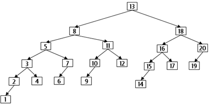
But what about an AVL tree? Let’s consider the "least efficient" AVL tree, namely, where every node is out of balance in one direction. These worst case trees have been studies and there is even a name for them: Fibonacci Trees.

These structures are named appropriately. The topmost root node has a left-subtree with 12 nodes while the right-subtree has 7 nodes.
Can you see that these numbers are both one less than a Fibonacci number (1, 1, 2, 3, 5, 8, 13, 21, ...). While these trees are balanced according to the AVL property, in the worst case, finding the minimum value will require the most work.
Observe how the effort reduces: First you search in a tree with 20 nodes, then the left sub-tree has 12 nodes, then the left grandchild-tree has 7 nodes, and so on. While not subdividing "in half" as one needs to do (such as for binary array search) this subdivision is based on a different constant, called phi which equals (sqrt(5) + 1)/2 or ~1.61803
Yep, the golden ratio is at play. Illuminati confirmed.
So in this worst case, the problem is subdivided not in half but by 1.61803. How does this translate into our concepts? Or in other words, given any Fibonacci tree of N nodes, N+1 is a fibonacci number, how many times will the min() method recurse until it finds the smallest key?
You should be able to see that you can divide N by phi a total of log (in base phi) of N. Using basic principles of logarithms, this value is equal to log2(N) / log2(phi).
Note that log2(phi) = 0.694241...
So this crude analysis suggests that in the worst case, you can find the minimum in (1 / 0.694241) * log2(N) or 1.44 * log2(N).
Let’s double check. In this example with 20 nodes, there are five edges to get to the minimum or a recursion of 5. This formula predicts it will not be greater than 6.22. Trying this on larger values of N will show that the formula is a good predictive model.
In any event, the most important result is that we have an upper bound on the total number of recursions in terms of some constant multiplied by log2(N), and we can use this to clarify that in this worst case, the performance is O(log N).
1.4 Empirical Evidence
You will routinely execute your programs and then graph its progress to determine how it will perform with larger and larger problem sizes. We now complete the description of the mathematical tools you need to properly classify the performance of your algorithms.

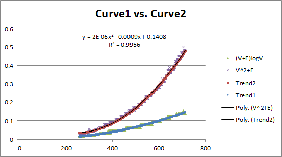
These two curves reflect two different algorithms. Observe that they have different growth behaviors. Is it possible to model these growth curves mathematically?
The performance of the algorithm (on average) appears to be hitting the mark very close to expected. But what happens in the worst case? Indeed, what is the worst case for each of these algorithms?
We want to be able to identify three cases for each algorithm:
best case – the situation in which the algorithm performs the least amount of work.
worst case – the (often pathological) case in which the algorithm must perform the most amount of work.
average case – using statistics and randomness, try to come up with an average problem size to use for expected performance.
For the duration of this lecture, we will be solely interested in worst case performance.
1.5 Major concerns
We started with Sedgewick’s Tilde expressions to rapidly approximate the execution performance of an algorithm, or to compute the number of times a key function (such as compareTo) executed. We then moved to a more loose description, I called "Order of Growth".
The goal was to evaluate the worst case behavior that would result for an algorithm and to classify the algorithm into a well known performance family. We have seen several of these families to date. We classify their order of growth (in the worst case) using the following notation:
Constant: O(1)– Time to complete is independent of the size of the data
Logarithmic: O(log n) – Time to complete is directly proportional to the log2 of the size of the data
Linear: O(n) – Time to complete is directly proportional to the size of the data
Linearithmic: O(n log n) – Time to complete is directly proportional to the size of the data times the log2 of the size of the data
Quadratic: O(n2) – Time to complete is directly proportional to the square of the size of the data
Cubic: O(n3) – Time to complete is directly proportional to the cubic of the size of the data
Polynomial: O(nk) – Time to complete is directly proportional to some constant power of the size of the data
Exponential: O(kn) – Time to complete is directly proportional to a fixed constant raised to a power directly proportional to the size of the data
But what does this terminology mean? we need to turn to asymptotic complexity to answer that question:

The above picture has a curve f(n) that represents the function of interest. At various times in this course, we have used this for a number of investigations:
Number of array inspections.
Number of times two object are compared with each other.
Number of times two values are exchanged during a sort.
We are increasingly interested in the performance of the overall algorithm, that is, instead of focusing on a single key operation, we want to model the full behavior so we can come up with a run-time estimate for completion.
The value n represents, typically, the problem size being tackled by an algorithm. As you can see, the value of f(n) changes over time, increasing when n increases. Here, n is the problem size.
The goal is to classify the rate of growth of f(n) and we use a special notation for this purpose, which looks awkward the first time you see it.
There are three notations to understand:
Lower Bound Ω(g(n)) – after a certain point, f(n) is always greater than c1*g(n).
Upper Bound O(g(n)) – after a certain point, f(n) is always smaller than c2*g(n).
Tight Bound Θ(g(n)) – after a certain point, f(n) is bracketed on the bottom by c1*g(n) and on the top by c2*g(n).
The phrase "after a certain point" eliminates some of the "noise" that occurs when working with small data sets. Sometimes even the most efficient algorithm can be outperformed by naive implementations on small data sets. The true power of an algorithm only becomes realized as the problem size grows to be sufficiently large. The constant n0 refers to the point after which the computations have stabilized. This value can never be uniquely determined, since it depends on the language used, the computer processor, its available memory, and so on. However, we define that it must exist (and it can be empirically determined for any algorithm should one wish to).
Note: We can use Ω(), Θ() and O() to refer to best case, average case, and worst case behavior. This can be a bit confusing. The whole point is to classify an asympotic upper (or lower) bound.
That being said, the most common situation is to analyze the worst case analysis. Since this is so common, most of the time it is understood. When I say, "Algorithm X is O(f(n))" I mean "the complexity of X in the worst case analysis is O(f(n))". This means that its performance scales similarly to f(n) but no worse than f(n).
Here is a statement that is always true: Everything that is Θ(f(n)) is also O(f(n)).
Once an algorithm is thoroughly understood, it can often be classified using the Θ() notation. However, in practice, this looks too "mathematical". Also it can’t be typed on a keyboard.
So what typically happens is that you classify the order of growth for the algorithm using O(g(n)) notation, with the understanding that you are using the most accurate g(n) classification.
To explain why this is necessary, consider someone who tells you they have a function to find the maximum value in an array. They claim that its performance is O(2n). Technically they are correct, because the rate of growth of the function (which is linear by the way) will always be less than some constant c*2n. However, there are other classifications that are more accurate, namely O(n).
And it is for this reason that all multiplicative and additive constants are disregarded when writing O() notations. Specifically, the constants matter with regard to the specific runtime performance of actual code on specific problem instances. Programmers can improve the code to reduce the constants, that is, making the program run faster in measurable quantities. However, theoretically, there are limits that programmers can achieve. And the overall order of growth, or rate of growth, is fixed by the design of the algorithm.
1.5.1 Order of Growth
Up until now, we were primarily concerned with order of growth analysis because that would help us to "eliminate the constants". Consider that you classifiy a function as requiring C(n) = 137*n2 comparison operations.
As the problem size doubles, then you would see C(2n) = 137*(2*n)2 comparisons. If you divide C(2n)/C(n) then the result eliminates the constants, resulting in 4. This is the hallmark of a quadratic behavior – when the problem size doubles, the result is a 4-fold increase.
We need to make one final comment on additive constants. If C(n) = 85*n + 1378, then C(2n) = 85*2*n + 1378. As you can see from the following table, ultimately the factor of n overwhelms the constant 1378. In fact, regardless of the magnitude of the constant, it will be overwhelmed by n once the size of the problem grows big enough.
n 85n+1378 C(2n)/C(n) 2 1548 4 1718 1.109819121 8 2058 1.19790454 16 2738 1.330417881 32 4098 1.496712929 64 6818 1.663738409 128 12258 1.797887944 256 23138 1.887583619 512 44898 1.940444291 1024 88418 1.96930821 2048 175458 1.984414938 4096 349538 1.992146269 8192 697698 1.996057653 16384 1394018 1.998024933 32768 2786658 1.999011491 65536 5571938 1.999505501
1.6 Asymptotic Analysis
You can find a wealth of information on Algorithms on the Internet. This Khan Academy Algorithms presentation is of higher quality:
In particular, you can start with
1.7 Big O Notation Cheat Sheet
Big O Cheat Sheet contains a summary of the information for various algorithms and data structures we have seen so far.
1.8 Version : 2023/04/17
(c) 2023, George T. Heineman
