CS 2223 Nov 30 2015

Lecture Path: 18
Back Next

Expected reading:
Daily Exercise:

The key to keeping your balance is knowing when you’ve lost it.
Anonymous

1 Final Half of Course

1.1 Getting Started

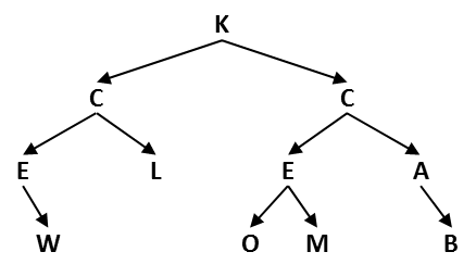
To get started, conduct a post-order traversal of the following tree. That would look like the following:

1.2 Balanced Trees

Today we will discuss how to automatically balance Binary Search Trees so they retain their efficiency.

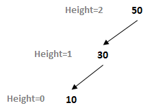
It is easy to see that a BST can become out of balance. Just consider adding three values to a tree in descending order, such as 50, 30, and 10. The resulting tree skews to the left as shown below:

One way to describe this skew is to identify two paths from the root to any root, whose lengths are noticeably different. Here, there is a path of length 2 from 50 - 30 - 10, and there is also a path of length 0 from 50 to the right (note there is no right child of root).

Once again, note how the height of a node in a BST is computed based on the maximum distance from that node to any of its descendants. Thus a binary tree with a single root node (with no children) would have height zero.

A balanced tree for these same values would look like the following:

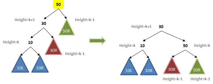
At a glance it looks quite different, but if you inspect its internal structure you can see there is a similarity. Indeed, let’s fill in some values and see if there is a pattern of behavior that we can exploit.

In this extended example, the BST has additional nodes, and the colored triangles describe collections of values. Note that the root node has a left subtree whose height is k+1 while its right subtree has a height of k-1. Having just this small imbalance is enough to begin the process of degrading the overall performance.

The technique of self-balancing a tree was discovered in 1962 by Adel’son-Vel’skii and Landis and it first appeared in a Russian mathematical journal. In CS this balancing binary search tree is known as an AVL tree.

An AVL Tree guarantees the AVL Property, namely, that the height difference for any node is -1, 0 or +1.

Assuming the above property holds, then the AVL tree is considered to be balanced. An AVL tree can become unbalanced by inserting or removing values from the tree. So you need to take care to properly correct whenever you observe that the tree has become unbalanced.

Remember the first time I introduced the BST that each node maintained an attribute, N, that reflected the number of values in the subtree rooted at that node? The original BST code had to properly compute N as each recursive invocation completed.

We will do the same thing. Upon observing an unbalanced node somewhere in the BST, special logic will be introduced that will correct the imbalance according to the AVL Property.

1.3 Four Scenarios

Given three values to be inserted into a BST, there are four imbalanced scenarios that need to be considered:

Each of these has a label associated with it that explains how to correct the imbalance. The case we covered earlier is known as Left-Left because of the relationship betwen these three values.

RotateRight operation

Let’s define an operation on a Binary Tree node called Rotate Right which adjusts the relative heights to conform to AVL. In this example, we can "lift" up 30 to effectively replace 50 as the root, and 50 is demoted to be a right child of 30.

Regardless of where the 50 node exists within a BST, the rotate right operation will properly rebalance the tree below it to conform to the AVL property. Naturally you have to continue working back up to the root as the recursion unwinds to make sure that successive ancestors also remain balanced.

As you can see from the sample code, each rotation operation is a fixed number of operations, so it can be considered to be constant. Since the height is now guaranteed to be ~log N, we have delivered on our promise for efficient BST data structures.

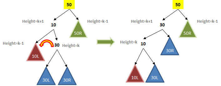
Let’s cover one of the more complicated examples, namely the Left-Right scenario. It isn’t enough to conduct a single rotation; you actually have to do two rotations:

As you can imagine, first a left rotation is performed to move the 30 up and the 10 down. Then a Right rotation is performed to lift the 30 up and move the 50 down. All corresponding subtrees are also adjusted.

The key to efficient AVL implementation is that each node stores its height value so it doesn’t have to be computed each time.

1.3.1 Red Black Trees

The Red Black Tree as describesd in pp. 424-437 is excellent. To be honest, this was the first time that I was able to fully understand Red Black trees. The key points you need to understand are:

AVL trees enforce a strong global property, namely, that the heights for left and right subtrees are never more than -1, 0 or 1. If you relax this restriction, you can reduce the number of rotations.
A RedBlack tree guarantees that no path to a leaf node is more than twice as long as any other path to another leaf node. This is strong enough to guarantee the desired properties.
RedBlack trees therefore allow for less compact trees, which increases the search time slightly, but it noticeably reduces the time to perform insertions and deletions.