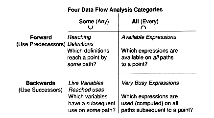
Data flow analysis provides information regarding the definition and use of data items. It provides the following information (among other): (1) paths along which a reference to a data item is not preceded by a definition and (2) detection of redundant or useless code. As the diagram above shows, we approach data flow analysis in two ways. The first, a low-level approach, is from a compiler phase perspective, using the control flow graph intermediate representation developed in Chapter 8. The second, a high-level approach, is to evaluate attributes on the abstract syntax tree.

Example 1 shows some problems which may be exposed by data flow analysis.

EXAMPLE 1

(1)

x := 3 (unused definition)

x := 2

(2)

x := 3 (useless assignment)

(no ... := x)

(3)

A := 3 (identical variables)

B := 3

In addition to those shown in Example 1, loop invariant variables may be detected, expressions which have already been computed may be detected, etc.

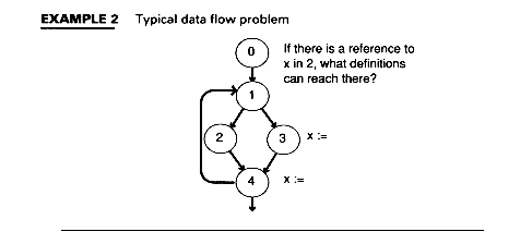
Most data flow problems can be defined by equations. Iterative techniques are used to solve these equations. Example 2 shows a typical problem.

EXAMPLE 2 Typical data flow problem

Given a control flow structure, we want to discern which definitions of program quantities can affect which uses within the program.

Data flow problems fall into two classes. First are those which, given a point in the program, ask what can happen before control reaches that point--that is, what (past) definitions can affect computations at that point. We call these forward flow problems.

Second are those which, given a point in the program, ask what can happen after control leaves that point--that is, what (future) uses can be affected by computations at the point. We call these backward flow problems.

Forward flow problems include reaching definitions and available expressions. Backward flow problems include live variable analysis, very busy expressions, and reached uses.

We will examine these one by one.

Reaching definitions determine for each basic block B and each program variable x what statement of the program could be the last statement defining x along some path from the start node to B.

A statement defines x if it assigns a value to x, for example, an assignment or read of x, or a procedure call passed x (not by value) or a procedure call that can access x.

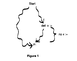
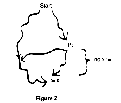
Formally, we say that a definition, def

def: x :=

reaches a point P in the program if there is some path from the start node to p along which def occurs and, subsequent to def, there are no other definitions of x. Figure 1 shows this pictorially.

For data flow analysis problems, we create and solve a collection of data flow equations. The variables are

In (B) and Out (B)

for a given block B.

There are two classes of equations:

1. A transfer equation to transfer data within the blocks

2. A confluence rule to transfer data when paths come together

For all forward flow problems, the information which comes out of the block is a function of the information which goes into the block. We write this symbolically as:

Out (B) = f_B(In (B))

For reaching definitions, we define function f in terms of definitions which are generated and killed in the block B. We thus introduce two new variables:Kill(B) and Gen(B).

Definition def₁ kills definition def₁ and def₂ define the same variable:

Kill (B) = The set of definitions in the other blocks of the program that are killed by some definition in B.

Block B generates definition def if def is in B and is the last definition of def's variable within B.

Gen(B) = set of definitions generated by B

The transfer equation is:

Out (B) = (In(b) - Kill(B)) Gen (B)

Confluence Rule for Reaching Definitions

A definition def reaches the beginning of a block B if and only if it reaches the end of one of block B's predecessors.

In(B) = Out(P)
_{P Pred(B)}

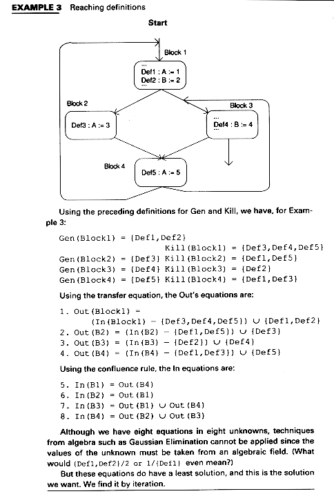
We will develop an iterative algorithm for reaching definitions. The reader need not despair that there will be a new algorithm for every data flow problem, however. Only minor changes need to be made to the equation to solve the other problems.

We start by assuming that what comes out of a block consists of the definitions generated in them.

We then repeatdly visit the nodes, applying the confluence rules to get new In's and the transfer rules to get new Out's. By pred(B), we mean the immediate predecessors.

Algorithm

Reaching Definitions

 FOR each block B, DO
   In(B) = 
   Out(B) = Gen(B)
 ENDFOR
   WHILE there are changes DO
     FOR each block B DO
       In(B) =  Out(P)
             P  Pred (B) 
       Out(B) = (In(B) - Kill(B))  Gen(B)
     ENDFOR
   ENDWHILE 

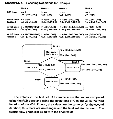
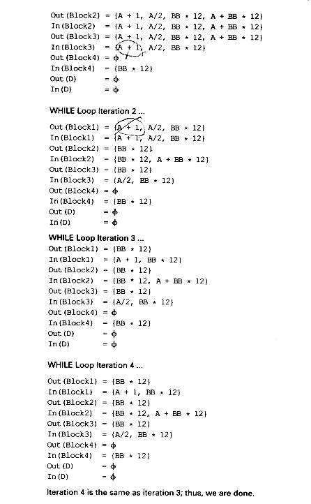
The values in the first set of Example 4 are the values computed using the FOR Loop and using the definitions of Gen above. In the third iteration of the WHILE Loop, the values are the same as for the second iteration; thus there are no changes and the final solution is found. The control flow graph is labeled with the final result.

Most of the space for these is devoted to storing the In(B) and Out(B) sets. These sets are a subset of all variable definitions.

We could represent a definition by a pointer to its text, but the In, Out sets may be large.

A better way is to number the definitions and create a table whose ith entry points to the ith definition. The In and Out sets can then be bit vectors such that the ith position is set if the ith definition is in the set.

Other space improvements include limiting the variables to be considered and then we can limit the length of the bit vectors.

For the bit vector operations, union can be implemented by a Boolean or, intersection by and, and set difference by and not.

Not all uses of data flow analysis involve code optimization. We can use reaching definitions to detect possible uses of variables before they have been defined. Detecting (at compile time) statements that use a variable before its definition is a useful debugging aid.

To adapt reaching definitions to solve this:

(i) Introduce a new dummy block D that contains a definition of each variable used in the program.

(ii) Place D before the Start node.

(iii) Compute reaching definitions.

(iv) If any definition in D reaches B where the variable is used, then we have a use before a definition.

In some languages, we should print a warning. In other languages, however, a default initial value may be assumed, and although a warning message could be issued, it would be incorrect not generate the code for the program.

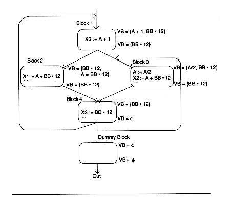
Available expressions make use of an expression used in one block which was computed in another block. Thus, at code generation time, code to recompute the expression need not be emitted. Example 5 shows an expression BB*12 which is computed on all paths leading to X3.

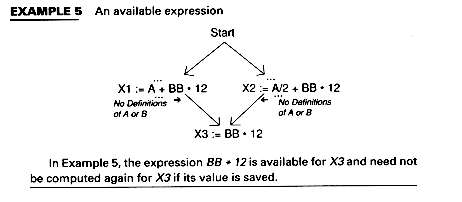
In Example 5, the expression BB*12 is available for X3 and need not be computed again for X3 if its value is saved.

Finding available expressions is similar to finding reaching definitions. Again we use the variables In(B), Out(B). We use the term A op B to mean any expression, even one which has more that one op, as in A + BB * 12.

Transfer Function Rules

For available expressions, the variables Kill(B) and Gen(B) are defined as follows:

Kill(B) = {the expressions X op Y in the program such that X or Y is defined in B},

that is, X or Y occurs on the left of an assignment statement or in a read statement.

Gen(B) = {the expressions X op Y computed in B, with no subsequent definitions of X or Y in B}

EXAMPLE 6 Gen and Kill sets for a block B

Consider the following statements in some basic block B

A := B + C
X := Y - Z
B := X + Y
X := A * B
In Example 6, Gen(B)={Y-Z, A*B}. Kill(B)={B+C,X+Y} plus other expressions such as, say, X + Q, since X is on the left-hand side of an assignment in B.

---

Transfer Equation

We have "rigged" the definition of Gen and Kill for available expressions so that the equation of Out is the same as that for reaching definitions

Out(B) = (In(B) - Kill(B)) Gen(B)

Confluence Rule

An expression is available at a point only if it is computed on all preceding paths:

In(B) = Out(P)

^{P Pred(B)}

We initialize In(start) = even though it may have predecessors.

Solving the Equations

This time we want the largest solution since we don't want to rule out an expression unless we find a path along which it is unavailable. Thus, we will initialize the In and Out sets to make every expression available and then eliminate expressions that are not readily available. Here, we throw things out (via intersection) the way reaching definitions threw things in (via union).

Algorithm

Available Expressions

 In(Start) = 
 Out(Start) = Gen(Start)
 FOR B < > Start DO
   In(B) = All Expressions in program
   Out(B) = (In(B) - Kill(B))  Gen(B)
 ENDFOR
 WHILE there are changes DO
   FOR B < > Start DO
     In(B) =  Out(P)
           P   Pred(B)

     Out(B) = (In(B) - Kill(B))  Gen(B)
   ENDFOR
 ENDWHILE 

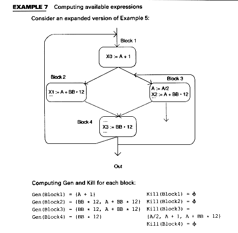
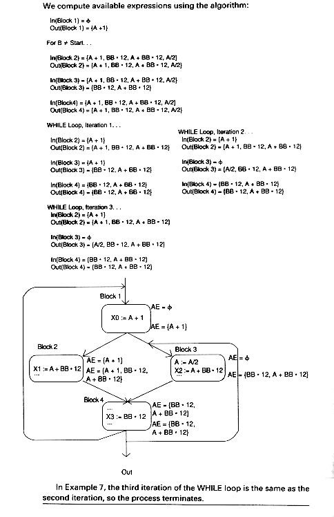
Available expressions eliminate recomputations. For example, suppose In(B) contains an expression A op B as does B₄ (BB * 12) in Example 7, that is, A op B is available at the beginning of the block as is BB * 12 at the beginning of block B₄. Suppose, further, that A op B is used in B (before A or B is redefined). Then we can avoid recomputing A op B in the following way:

1. Find all definitions that reach B and have A op B on the right-hand side.

2. Create a new variable T to hold the value of A op B.

3. Replace each definition Z := A op B from (1) by

T := A op B

Z := T

4. Replace all uses Q := A op B by Q := T.

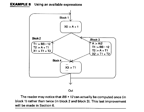
Example 8 shows this for the program of Example 7 and for the expressions BB * 12 and A + BB * 12.

Live variables at a program point P are those for which there is a subsequent use before a redefinition.

We compute live variables for a number of reasons. If there is a definition not followed by a use, then we may want to issue a warning message to the programmer.

Even if there is no definition at a program point P, we may want to keep track of what variables are live to know which ones to keep in registers. If the variable is not to be kept in a register, we may want to store it to reuse the register, but if the variable is not live, we do not need to store it; that is, the code generator does not need to emit a store instruction.

Formally, we define a variable to be live at some point in the program if there is some path through the flow graph from that point along which we shall encounter a use of that variable before any redefinition; otherwise, the variable is dead

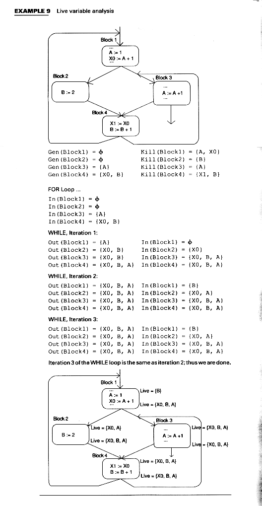
The equations for live variables resemble those for except that the data "flows backwards" from the Out's to the In's rather than from the In's to the Out's. Note that In still refers to the "top" of a block and Out to the "bottom", with "top" referring to the part of a block where there is the head of an arrow, and "bottom" meaning a tail.

Transfer Equation New information transfers from the end to the beginning of a block. We define Gen and Kill, however, as follows:

 Kill (B)  : {variables defined in B} Gen (b)  : {variables used before a redefinition in B}  In(B) = (Out(B) - Kill(B))  Gen(B) 

Confluence Rule The confluence rules for back wards flow are really "divergence rules".

 Out (B) =  In(S) 
 S  Succ(B)

 
 

This time, we once again want the smallest solution -- we don't say a variable is live unless we actually find a path along which it is used before being redefined.

Thus, we start by assuming nothing is live on exit from any block. The process stops because we are only adding variables to the sets (and there are a finite number of variables).

Algorithm

Live Variable analysis

 FOR all blocks B DO
   IN(B) = Gen(B)
 ENDFOR
 WHILE there aer changes DO
   FOR each block B DO
     Out(B) =  In(S)
         S  Succ(B)
     In(B) = (Out(B) - Kill(B))  Gen(B)
   ENDFOR
 ENDWHILE 

The ideas are the same as for reaching definitons. We can identify variables with positions in a bit vector, using a table of pointers (perhaps to the symbol table) to make the association.

Reached uses is a similar problem to live variable analysis.

A Use of A is reached from the assignment statement A := if there is some path from the assignment to the use along whitch A is not redefined.

We can detect useless assignments: they are those assignments with no reached uses.

To find the equations for reached uses, note that the last definition of A in a block B reaches what the end of block B reaches, plus subsequent uses of A within B. Prior definitions of A within B reach only their uses within B.

Equations for Reached Uses

The domain is somewhat different here: the set of pairs consisting of a statement S and a variable A appearing on the right of S.

Kill(B) = {(S,A) | S not in B and B contains an assignemnt to A}

Gen(B) = {(S,A) | S B, A on right-hand side of S, and no definitions of A prior to S in B}

Transfer Equation

In(B) = (Out(B) - Kill(B)) Gen(B)

Confluence Equation

Out(B) = In(S)
S Succ (B)

The algorithm is essentially the same as that for live variables; that is, we assume nothing is reached, and apply the equations. The result is the smallest solution since a use is reached only if we can really find a path to it.

An expression A op B is very busy at a point p if along every path from p there is an expression A op B before a redefinition of either A or B.

If an expression is very busy at program point p, it makes sense to compute it there. This is often termed code hoisting and it saves space although it doesn't necessarily save time.

But it is interesting as a fourth type of data flow analysis problem: backwards flow and intersection confluence.

 Kill(B) = { X op Y | either  X or Y defined before use of x op Y in B}
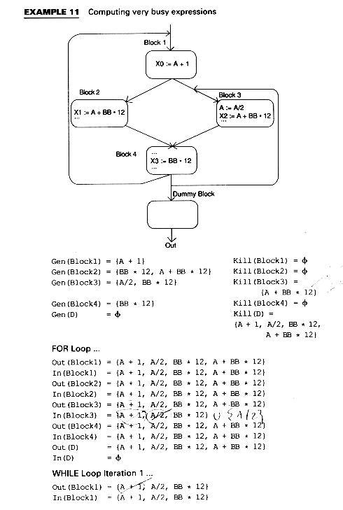
 Gen(B) = {x op Y |  X op Y used in B before any definition of X or Y} 

Transfer Equation

 In(B) = (Out(B) - Kill(B))  Gen(B) 

Confluence Equation

 Out(B) =  In(S)
 
 S  Succ (B)

 
 

Algorithm for Computing Very Busy Expressions

We want to avoid considering X op Y as very busy just because neither X nor Y is redefined. To do this, we introduce a dummy block D such that

 Kill(D) = all expressions
 Gen(D) = none 

and we let D be a successor of all blocks that have the program end as a possible successor.

Algorithm

Very Busy Expressions

 FOR each block B DO
   Out(B) := all expressions
   In(B) := (Out(B) - Kill(B))  Gen(B))
 END
 WHILE there are changes DO
   FOR each block B DO
   Out(B) =  In(S)
 
 S  Succ (B)
 
 
   In(B) = (Out(B) - Kill(B))  Gen(B)
 ENDFOR
 ENDWHILE 

We can perform data flow analysis on a tree when the tree is known to represent the program flow(e.g., no multiple entries and exits from loops, no GOTO's etc.).

The following live variables analysis is described by Babich and Jazayeri (1978a). They compute dead variables and available expressions. We will discuss dead variables. Exercise 9 asks the reader to write the equations for available expressions and reaching definitions.

A variable is defined as dead at a point in a program if its value will not be used after control leaves that point.

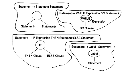
The following (ambiguous) grammar will be used:

 Statement  Statement1 Statement2

 Statement  IF Expression THEN Statement1 ELSE Statement2

 Statement  WHILE Expression DO Statement

 Statement  Label : Statement

 Statement  GOTO Statement

 Statement  Assignment

 Statement  ReadStatement

 Statement  WriteStatement

 

The following notation will be used for the tree nodes:

Four Boolean attribute, Kill, Gen, DeadAtBeginning and DeadAtEnd, will be associated with each of these nodes. For simplicity, only one variable will be analyzed. Exercise 7 asks the reader to extend this for more than one variable. The equations will reflect the following:

Statement.DeadAtBeginning := True if the variable is Dead at the beginning of Statement.

Statement.DeadAtEnd := True if the variable is DEAD at the end of Statement.

Statement.Kill := True if the variable is assigned a value in Statement.

Statement.Used := True if the variable is used and not assigned in Statement or else used in statement before being assigned in Statement.

We will define these first two more precisely below. The algorithm will iterate because none of the methods we have developed so far will work (see Exercise 6).

Since deadness at a point is inherently a property of the portion of the program that comes after that point, we need to have sacnned the portion of the program that that node. Thus, we scan the tree from right to left.

The attributes DeadAtBeginning and DeadAtEnd are defined as follows:

For Assignment, Read, and Write Statements:

Statement.DeadAtBeginning := NOT(Statement.Used) AND (Statement.Kill|Statement.DeadAtEnd)

For Statement Statement₁ Statement₂, we note that we want to start with the value of Statement.DeadAtEnd and compute Statement.DeadAtBeginning and that the end of Statement₁ is also the beginning of Statement₂. Therefore,

 Statement2.DeadAtEnd := Statement.DeadAtBeginning

 

and since the end of Statement₁ is also the beginning of Statement₂,

 Statement1.DeadAtEnd := Statement2.DeadAtBeginning

 

The beginning of Statement₁ is the same point as the beginning of Statement, so:

 Statement.DeadAtEnd := Statement1.DeadAtBeginning

 

The equation for IF statements and WHILE statements are similar. The attribute grammar is:

 (1) Statement  Statement1 Statement2

   (i) Statement2.DeadAtEnd := Statement.DeadAtBeginning

   (ii) Statement1.DeadAtEnd := Statement2.DeadAtBeginning

   (iii) Statement1.DeadAtEnd := Statement2.DeadAtBeginning

 

 (2) Statement  IF Expression THEN Statement1 ELSE Statement2

   (i) Statement2.DeadAtEnd := Statement.DeadAtEnd

   (ii) Statement1.DeadAtEnd := Statement.DeadAtEnd

   (iii) Statement.DeadAtBeginning := NOT (Expression.Used)

 	AND (Statement1.DeadAtBeginning AND Statement2.

 	DeadAtBeginning)

 

 (3) Statement  WHILE Expression DO Statement

   (i) Statement.DeadAtEnd := NOT (Expression.Used) AND 

 	(Statement.DeadAtEnd AND Statement1.DeadAtBeginning)

   (ii) Statement.DeadAtBeginning := NOT (Expression.Used) AND 

 	(Statement.DeadAtEnd AND Statement1.DeadAtBeginning)

 

 (4) Statement   Label : Statement

   (i) Statement1.DeadAtEnd := Statement.DeadAtEnd

   (ii) Statement.DeadAtBeginning := Statement1.DeadAtBeginning

 

 (5) Statement   GOTO Statement

   (ii) Statement.DeadAtBeginning := TargetStatement.DeadAtBeginning

 

 (6) Statement   Assignment | ReadStatement | WriteStatement

   (i) Statement.DeadAtBeginning := NOT (Statement.Used) AND

 	(Statement.Kill | Statement.DeadAtEnd)

 

 

For the WHILE loop the rules for Statement₁.DeadAtEnd and Statement.DeadAtBeginning are the same because an exit from the body of a WHILE loop is followed by a branch back to reenter the loop.

It may be necessary to compute the attributes at a node more than once before the correct values are computed. The (recursive) algoritm to compute attribute values for each statement is:

Algorithm

Dead (statement)

 BEGIN {Dead}

 FOR each component of Statement,

     in right to left order,

 BEGIN

   Compute Component.DeadAtEnd

   Call DEAD (Component)

 END

 Compute Statement.DeadAtBeginning

 END {Dead}

 

The values for DeadAtEnd and DeadAtBeginning are saved in the tree as they are computed. Thus each tree node contains at least the following information:(1) node type (compound, IF, WHILE, etc.), (2) the values of DeadAtEnd and DeadAtBeginning, (3) assorted pointers to other nodes, describing the position of the node in the tree and (4) values of Used and Kill where needed.

In a pass over the tree, attributes whose values are needed will usually be computed before they are used. In two cases, however, this will not be true. The first case is backward GOTO's since the right to left scan will not have computed the right-hand side of the semantic function. The second case is for WHILE statements since to find DeadAtEnd, we need DeadAtBeginning, which isn't know because Statement₁ hasn't been analyzed yet. Because of these two cases, we initialize these attributes to True.

The evaluation algorithm iterates until no attribute value changes.

Algorithm

Dead(Tree)

 While there are changes to any attribute value DO

   Initialize attributes to True

   BEGIN

     Store Root.DeadAtEnd and Call Dead(Root)

     Store any changed values

   END

 

Example 12 shows a program and the values after two passes over the tree, analyzing the attribute values for the variable A.

EXMAPLE 12 High-level data flow analysis example

 Read A

 WHILE B < > 0 DO

   BEGIN

     Write A

     WHILE A < 5 DO

       BEGIN

         A := A + 1

         Write A

         B := A

       END

     Read (A)

   END

 

Pass 0( Initializing Attributes to True):

Pass 1

Example 12 shows the initialization pass and pass 1 of the evaluation. The reader is asked to perform the remaining passes in Exercise 8.

The preceding sections have discussed intraprocedural data flow analysis, that is, data flow analysis within a procedure. Interprocedural data flow analysis discusses the same issues, but with intervening function or procedure calls. this is shown below, where we might ask if expression X + Op Y is available. If function f does not modify either x or y, then it will be available.

 A : X + Y

 ...

 Y := f(A)

 ...

 B := X + Y

 

One method is to assume a worst case: no expressions will be available after a subprogram call, no variables are live, etc.

To perform a more accurate interprocedural data flow analysis, we need to calculate the call chain, that is, what subprograms are called within a subprogram.

Interprocedural analysis often involves finding aliases. A variable X is an alias of a variable Y if X and Y are different names for the same memory location. Reference parameters are an example of aliasing, as are assigning the value of one pointer to another. Thus, changing one of the variables effectively changes the other.

For languages which require explicit declaration of global variables and reference parameters, it may be reasonable to perform an interprocedural analysis. Reference parameters and globals which are changed in the procedure may be identified via Gen and Kill sets.

Changes to any element of an array are usually recorded as having changed the entire array since it may be impossible to tell at compile time which element will be changes.

This chapter discussed data flow problems, at first on the low-level control flow graph and then on an abstract syntax tree representation. Data flow problems can be divided into two types: backwards flow problems and forward flow problems. They can also be partitioned into problems whose confluence rules use union and those which use intersection. The following figure shows the five problems discussed in this chapter in these categories:

We will use data flow analysis in the next chapter when we discuss specific examples and specific optimization categories.

In Chapter 12, we will look at data flow analysis again when we discuss incremental compling.