[WPI] [cs2223] [cs2223 text] [News] [Syllabus] [Classes] 

cs2223, D97/98 Class 25

Non-uniform probability distributions

In Class 22 we showed how to obtain uniformly-distributed "random" numbers. Sometimes we need non-uniformly distributed random numbers. The usual way to specify the uniformity of the distribution is by means of a probability distribution function. The probability distribution funtion for uniformly distributed random numbers in the range 0->1 looks like this:

The probability distribution function doesn't directly show anything which is measurable. However, if we look at a small region about x, it tells us that the probability - which is equal to the fraction of the total cases - of a random value lying within that region is proportional to the width of the region:

The actual definition of P(x) is a differential one:

The function P(x) is just the proportionality constant at each value of x. The height of the function P(x) doesn't matter for our purposes, but by probability theory, it's integral has to equal one (which corresponds to all of the possible cases of numbers:

The graph above shows that the uniform distribution means that the same number of "random numbers" appears in any small band of values. Suppose, however, that we want to generate non-uniformly distributed numbers. For example, the lengths of e-mail messages and the times of day at which they are sent are not uniformly distributed. A numerical simulation of a mail server is more realistic if our "randomly"-generated e-mail messages have the same statistical properties as the e-mail. Here is one way to do that.

Suppose we have a function which returns the desired probability distribution, P(x).

double P(double x); // prototype

Now draw an imaginary rectangle which completely encloses the function. We want the fraction of the "random" numbers in a small band beginning at x to be proportional to the value of P(x) at that point.

That quantity is proportional to the area below the curve P(x) at that point. So, we can modify our integration function from Class 22 to generate non-uniformly distributed random numbers.

double nurm(double a, double b, double c, double (*P) (double))
   {
   int counter = 0;
   do
      {
      double x = a + (b - a) * ((double) rand() / (double) RAND_MAX);
      double y = c * ((double) rand() / (double) RAND_MAX);
      }
   while (y > P(x));
   return x; 
   } // end nurm()

A random number pair is generated inside the rectangular box. Keep trying random pairs until one is found which lies under the curve P(x) and return the value of x. This algorithm may seem inefficient - some values are calculated then thrown out. However, the quantity of wasted numbers is proportional to the area inside the box but above the curve; if the rectangular box is chosen intelligently, the extra effort can often be minimized.

Graphs

A graph is a collection of nodes and edges which connect the nodes.

Edge Matrix

Many data structures are used to store graphs. One way is to store a matrix of edges where each value E_xy shows a connection from node x to node y:

A one shows two nodes are connected and a 0 shows there is no connection. The zeros along the main diagonal show that no nodes connects to itself. For an undirected graph such as this, the graph is symmetric - values are mirror-reflected about the main diagonal because each path is two-directional.

If the graph is directed,

then the edge matrix can be stored in several different ways.

The first has the advantage of only requiring e ones while the second has the advantages of being anti-symmetric

and of allowing one to determine all node connections, even the ones which cannot be traversed because the edges are directed.

It is easy to write algorithms for graphs stored this as edge matrices, but the storage and algorithms are inefficient, since they tend to be of order O(e²), where e is the number of edges in the graph. The number of ones in the matrix is e or 2e, which is almost always much smaller than ².

Node List

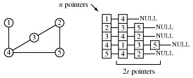
Another way to store a graph is as an array of nodes with pointers to linked lists of connecting nodes.

The order of the nodes in the linked lists doesn't matter. The size of the array is n, the number of nodes, and there are 2e pointers in the linked lists. Thus the number of pointers required to store the graph is

The average depth of the linked lists is

unless the graph is unusually pathological. An operation to address the beginning of any of the linked lists is of order O(1), constant time. Thus an algorithm which examines each edge is of order O(e) and one which searches for a particular connection to a particular node is of order O(1). This method of storing graphis is efficient, but requires more programming effort that edge matrices.

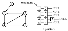
The node lists for directed graphs are even smaller.

Breadth-First Graph Traversal

Suppose we want to traverse a graph, for example, we want to print each node's value once. One way to do that is to pick an arbitrary node as a starting point and provide a means for marking each node as "touched" - which means "I've seen this node" or as "examined" which means "I've looked at each edge connected to this node".

Begin at node 4 and print its value as the node is touched. Now explore the node. Any new nodes which are touched (and printed as they are touched) are added to a queue.

Recursively pop a node from the queue and examine it. Any connecting nodes are put on the queue and printed - but only if they have not been touched or examined. When the queue is empty, every node has been examined and printed once, when it was first touched. Printing progresses from root to leaves.

print order: 4, 2, 3, 5, 1

This algorithm is called breadth-first traversal because each node is explored before it's children. Now redraw the graph keeping only the paths which were traversed.

Class 24.

Depth-First Graph Traversal

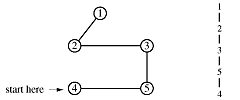
We change the above algorithm in two ways:

• Explore the children of each node before printing the node value.
• Use a stack instead of a queue.

'

print order: 1, 2, 3, 5, 4

Once again, the order of traversal produces a tree.

But, with depth-first traversal - so called because the farthest limits of the graph are explored and printed first - the trees tend to be narrow and deep and the leaves are printed before the root. The trees are equivalent to the post-ordered tree traversal discussed in Class 24.

Depth-first traversal is usually implemented recursively so no explicit stack is needed.

[cs2223 text] [News] [Syllabus] [Classes]

Contents ©1994-1998, Norman Wittels
Updated 26Apr98