[WPI] [cs2223] [cs2223 text] [News] [Syllabus] [Classes] 

cs2223, D97/98 Class 24

Trees

The tree is a useful data structure for describing an algorithm involving a sequence of decisions. A classical example is the N-queens problem. The queen is the chess piece which can move any number of spaces along its own row or column or along either of its diagonals.

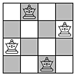
A queen can capture anything in any space into which it can legally move. This means that no two queens can reside stably on the same row, column, or diagonal. Suppose we want to arrange some number of queens in a stable configuration on a chess board. Here is an example of a solution to the 4-queens problem.

Suppose we want to create an algorithm which finds solutions to the N-queens problem. We can represent the choices as a tree:

The above solution is shown in red. Not every leaf of this tree represents a solution. For example, the left-most leaf represents a placement of all four queens on the same diagonal. However, we could construct this tree and eliminate (or mark) the branches which allow a queen to be captured. This requires an orderly way to traverse a tree, examining each path exactly once.

Traversing a Tree

There are two major ways to traverse a tree: pre-order traversal and post-order traversal. The difference is whether the algorithm examines a node's contents before or after examining the contents of all of its children. For example, suppose the tree is a binary tree of ints:

class node
	{
	int value;
	node *left;
	node *right;
	}

If we use the usual convention of using null pointers to signify a leaf, then we can write two class functions to print recursively the node and all of its children:

void node::pre_print()
	{
	cout << value << endl;
	if (left) left.pre_print();
	if (right) right.pre_print();
	}
void node::post_print()
	{
	if (left) sum+= left.post_print()();
	if (right) sum+= right.post_print();
	cout << value << endl;
	}

In the first case, the values are printed before the children are explored. Thus the root is printed first and then the rest of the values - those generally nearer the root before those farther from the root. The last value printed is a leaf.

In the second case, the values are printed after the children are explored. Thus a leaf is printed first and then it's parent and then the rest of the values - those generally farthest from the root before those nearer the root. The last value printed is the root.

The second function seems more wasteful of stack space - the function is recursively called as many times as possible before the first value is printed, but both algorithms are useful.

Ancestry

As an example, consider this algorithm for determining ancestry. It is easy to tell if one node is the child or parent of another, but suppose we have two nodes and we want to tell if one is the ancestor of the other. That means that the first node lies on the path between the second and the root of the three. In this tree, node

B is an ancestor of node F but not of node H, even though H lies at the same depth as F. Suppose we want to know whether B is an ancestor of F. We can start at F and work backwards from parent to parent until we reach the root, looking for B. If we don't find B then B is not the ancestor of F. There are two problems with this approach. First, it is expensive, especially if the tree is large. Second, it is not always easy to determine parentage, unless a parent pointer is included in each node.

One way to solve this problem is by preconditioning. We add two numbers to each node - the pre-order traversse order and the post-order traverse order of the node. We show the pre-order number on the left and the post-order number on the right:

Now consider the pre-order numbers of two nodes, x and y. If

then either of these cases is true.

• x is an ancestor of y
• or, x is to the left of y in the tree.

Thus 2<4 and B is an ancestor of I, even though I is to the left of B; 2<12 and B is left of but not an ancestor of L; 2<6 and B is both an ancestor and to the left of F. You can't tell which of the three cases is true, just that one of them is true.

Now consider the post-order numbers of two nodes, x and y. If

then either of these cases is true.

• x is an ancestor of y
• or, x is to the right of y in the tree.

If we combine the two conditions,

then x must be an ancestor of y. And, it takes only two comparisons to determine ancestory, so this algorithm is of order O(1), it has constant time. By comparision, the direct search method of going from parent to parent isof order O(lgn).

Preconditioning is a frequent tree operation. However, it is of order O(n), so it only makes sense if it reduces the order of some other operation to below O(n) or if the results will be used many times. Unfortiunately, any changes in the tree could require re-preconditioning.

[cs2223 text] [News] [Syllabus] [Classes]

Contents ©1994-1998, Norman Wittels
Updated 26Apr98