cs2223 Class 16

[WPI] [cs2223] [cs2223 text] [News] [Syllabus] [Classes]

cs2223, D97/98 Class 16

Matrix Operations

We briefly discussed the problem of matrix multiplication. See Section 7.6 in the text.

Matrix Terminology

Note, there are variations in matrix terminology. This terminology comes from an excellent introductory matrix book: AJ Pettofrezzo, Matrices and Transformations (1966, Dover), ISBN 0-486-63634-8.

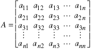
A matrix is a collection of numbers (ot other objects) arranged in rows and columns. The usual notation for a matrix element is two subscripts with row and column number, in that order.

Figure showing the matrix A whose elements are a11 in the upper left corner then a12, a13, ..., a1n across the top row; a21, a22, ..., a2n across the second row and so forth. The last row is an1, an2, an3, ... ann.

A square matrix is one with the same number of rows and columns. A is a square matrix.

Each matrix element has a comatrix, which is the submatrix formed by eliminating the element's row and column. Here are two comatrices of the matrix A.

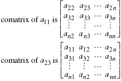
comatrix of a11 is {{a22, a23, ..., a2n}, {a32, a33, ... , a3n}, ... , {an2, an3, ... ann}}; comatrix of a23 is {{a11, a12, ... , a2n}, {a31, a32, ..., a3n}, ... , {an1, an2, ... ann}}

A matrix with only one row and column has no comatrix (or the comatrix is empty). The comatrix of a square matrix is also square, but the order of the matrix (number of rows and columns) is reduced by one.

There is an alternating sign associated with some matrix operations. It is calculated using the formuls

where r and c are the row and column numbers. This produces a sign which is positive in the upper left corner of the matrix and the sign changes with each step along a row or column. This can be represented by a sign matrix:

Figure showing a matrix with alternating signs. The top row is +-+-+-..., the second row is -+-+-+..., and so forth

Determinant

The determinant is a single number which characterizes a square matrix. It has a recursive definition. If a matrix is of order one (a single number), it's determinant is its value:

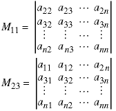
Note the use of the enclosing vertical lines | | to denote determinant. The minor of an element is the determinant of its comatrix:

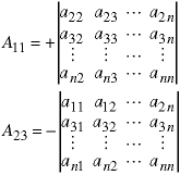
M11 = determ({{a22, a23, ... , a2n}, {a32, a33, ..., a3n}, ... , {an2, an3, ..., ann}}); M23 = determ({{a11, a12, ..., a2n}, {a31, a32, ..., a3n}, ... , {an1, an2, ... , ann}})

The cofactor of an element is its minor times the sign from the sign matrix:

A11 = +M11 and A23 = -M23, where M11 and M23 are given in the last equation

The determinant of a matrix of order n>1 can be written as a sum of determinants of order n-1. Specifically, it is the sum of the products of all of the elements in any row or column of the matrix times their respective cofactors.

|a| = sum(k=1->n; a1kA1k) = sum(k=1->n; a3kA3k) = sum(k=1->n; ak2Ak2)

These examples show the sum over the elements in the first row, the third row, and the second column, respectively. There are 2n such sums for a matrix of order n, and they all give the same value for the determinant. In practice, a program to calculate a determinant would pick a specific row or column - usually the first - for any matrix.

This algorithm is inherently recursive.

Analysis of the Determinant Algorithm

We used the determinant algorithm as an example of the summing factor method for solving recurrence relations, as discussed in the recurrence relation notes.

The algorithm for calculating the determinant of a matrix of order n forms the sum of n terms, each of which requires the calculation of the determinant of a matrix of order n-1. This leads to the recurrence relation for the "time" the algorithm takes:

The right sode of this equation can represent the n summations or the n increments in the loop which calculates the cofactors, etc. In fact, almost anything we include in the calculation will be of order n and we chose this value to make the solution easier. If you decide to change the right side of the recurrence relation, your calculation of the time will change somewhat.

This recurrence relation is linear and first-order, but the coefficients are not constant. Use the summing factor method with these definitions:

The initial condition states that no time is required to calculate the determinant of an empty matrix. We will need the product of the b_n.

prod(k=1->n; b(k)) = prod(k=1->n; k) = n!

The solution is:

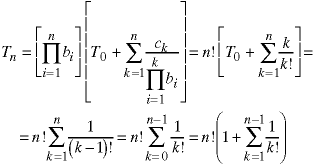
T(n) = prod(i=1->n; b(i)) * (T(0) + sum(k=1->n; c(k) / prod(i=1->k; b(i))) = n! * (T(0) + sum(k=1->n; k/k!) = n! * sum(k=1->n; 1/(k-1)! = n! * sum(k=0 -> n-1; 1/k! = n! * (1 + sum(k=1 -> n-1; 1/k!)

We can find an approximate answer for the last summation by using the Taylor series identity for e, the base of the natural logarithms.

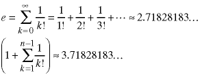
e = sum(k=0 -> infinity; 1/k!) = 1/1! + 1/2! + 1/3! + ... = 2.71828183...; (1 + sum(k=1 -> n-1; 1/k!) about= 3.71828183...

The time for the determinant algorithm is:

T(n) about= n! * 3.71828183...; O(T(n)) = O(n!)

Just how big is n factorial? The Stirling approximation is:

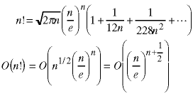
n! about= sqrt(2*pi*n) * (n/3)^n * (1 + 1/12n + 1/228n^2 + ...); O(n!) = O(n^(1/2) * (n/e)^n) = O((n/e)^(n+1/2))

How big is that last quantity? Where does it fit into the heirarchy of orders we studied in Chapter 2 of the text?

Try comparing it with

O((n/e) ^ n)

and with

O((n/A) ^ (n + 1/2))

for values of A that are both larger than e and smaller than e.