John Pawasauskas
CS563 - Advanced Topics in Computer
Graphics
March 18, 1997
This presentation deals with the topic of generalized unstructured decimation. First decimation will be defined and described, followed by decimation methods for several different types of images. The performance of the decimation process will be compared.
The material covered in this presentation was originally motivated by the need for efficient and accurate decimation of volume tessellations (unstructured tetrahedrizations). Pre-existing surface-based decimation schemes didn't generalize to volumes, so a new technique was developed, which allowed local, dynamic removal of vertices from an unstructured tetrahedrization while preserving its initial tessellation topology and boundary geometry.
Before proceeding any further, it is important to make sure that we understand the meaning of some of the terms which will appear in various places.
This presentation follows the format laid out in the paper "Generalized Unstructured Decimation" by Kevin J. Renze and James H. Oliver. The images which are incorporated in this presentation were taken from that paper. Some of the concepts which were difficult to understand, and in those cases where they were fundamental text may have been copied from that paper. Likewise, the algorithms which were presented by Renze and Oliver were copied directly.
The term decimation is used to describe the process of removing entities, such as polygons, from a geomatric representation. The goal of decimation is to significantly reduce the number of primatives required to accurately model the problem of interest, and to do so intelligently. Unstructured decimation algorithms came about primarily because of research into surface reconstruction.
There are a number of areas in which decimation can prove useful. Besides surface reconstruction, decimation may be useful in scientific and engineering applications. Decimation of polygonal surface models is especially useful in synthetic environment applications where large, complex models must be rendered at interactive frame rates (15 to 30 frames per second). Since models for synthetic environments are usually generated for other applications, such as CAD and medical imaging, they are not well suited for interactive display, since they typically are very large.
The basis for the algorithm is a unique and general method to classify a triangle with respect to a non-convex polygon. In other words, to determine whether the triangle lies inside or outside of the polygon. The decimation algorithm produced can be applied to both surface and volume tessellations, and is efficient and robust because it does not use floating-point classification calculations.
Surface decimation algorithms usually use either vertices, edges, or faces as the primative element to be removed. There are a number of different algorithms which can be used for surface decimation. None of them, however, apply to volume decimation. The basic concepts in two- and three-dimensional surface literature are extended to apply to unstructured volume applications.
The general decimation algorithm has several relatively simple steps. They are:
For 2D problems, such as planes or general surfaces, there are a number of algorithms which can be used to compute the new triangulation. In the case where only convex polygons are used, the problem is very easy to solve. Using an algorithm for triangulating star-shaped polygons, or using a constrained triangulation method such as a greedy triangulation algorithm, would be enough to solve the 2D tessellation problem. None of these algorithms seem to work in more than two dimensions, however. As Bern and Eppstein stated in their paper Mesh Generation and Optimal Triangulation, "There does not seem to be a reasonable definition of a constrained Delaunay tessellation in three dimensions.
Unconstrained Delaunay tessellations can be generalized to higher dimensions, but the result is always convex. If the initial local boundary loop is non-convex, some of the n-simplices which result will intersect valid n-simplices which are external to the local boundary loop. This violates the global tessellation. This requires that we implement an n-simplex classification system in order to handle non-convext regions.
The n-simplex classification problem has two possible solutions:
For angle summation we need an ordered boundary, and it may be restricted to 2D problems. Ray intersection algorithms can be applied to both 2- and 3-D problems, and additionally does not require an ordered data structure. However, ray intersection algorithms allow degenerate cases, such as when a ray is tangent to a boundary edge. An alternative method uses a postprocessing scheme which preserves the topology to classify the valid n-simplices.
The decimation algorithm needs an arbitrary collection of vertices as its minimum input. The connectivity doesn't need to be specified, but can instead be computed using any general tessellation algorithm. Non-convex geometry and topology with holes can be specified by explicitly specifying the vertex and connectivity information.
In order to determine how robust the algorithm is, extreme cases are tested. The conditions used are that each boundary vertex is retained, and each interior vertex is a candidate for removal. All non-boundary vertices can be deleted.
Most of the time, practical applications will use less severe decimation criteria. Criteria used to determine whether a vertex may be removed can be based on geometric properties or any scalar governing function specific to the application. Different criteria are usually required for rendering and analysis applications.
Given a planar tessellation, for each vertex v in the candidate decimation list:
Step two in the above algorithm generates a candidate tessellation and identifies the set of valid triangles that tessellate the hold created by vertex decimation. First create an unconstrained Delaunay triangulation over the set of adjacent vertices that define the local boundary loop. Every adjacent vertex is initially connected to the candidate decimation vertex v by an edge. The convex hull of the local triangulation loop may not coincide with the local boundary loop, so we must determine which candidate triangles lie inside the boundary. From this set we must determine the remaining interior triangles.
If all of the decimation criteria have been met for the candidate vertex, we can apply the following algorithm the hole which will be created by removing it:
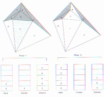
The above figure shows the contents of the Valid, Interior, and Exterior stacks corresponding to Phase 1 and Phase 2 of the classification algorithm described above. In this example, the local boundary loop encloses the triangles labeled 0, 1, 2, 4, and 5. Unshaded triangles denote that the triangle is on the Valid stack. Lightly shaded triangles reside on the Interior stack, and darker triangles reside on the Exterior stack.
In Phase 1, all successful classifications share one thing - each interior triangle exclusively shares at least one original boundary loop edge. Complex convex and non-convex geometry is the reason why Phase 2 of the classification algorithm is required. After Phase 1, we cannot determine whether triangles which share no original boundary edges should be members of the Valid stack. These elements are put on the Interior stack. Triangles which do not exclusively share at least one original boundary edge are put on the Exterior stack, to be considered in Phase 2.
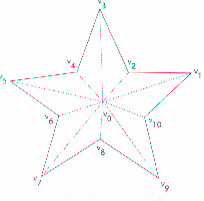
This local tessellation algorithm fails if an exclusively shared, original, local boundary loop edge does not exist in the local tessellation. This isn't an anomaly, which can be shown by a relatively trivial non-convex topology illustrated in the following figure. Since the Delaunay tessellation algorithm is guaranteed to return a candidate local tessellation bounded by its convex hull, Phase 1 of the classification algorithm will fail. The "failed" candidate decimation vertex will be queued for processing later. As soon as one of its adjacent vertices is removed, the "failed" vertex decimation candidacy is automatically renewed.
A general 3D surface decimation algorithm was developed based on the new planar decimation algorithm described above. To show a straightforward extension to surface decimation, Renze and Oliver implemented the local projection plane and the distance-to-plane criterion which was developed by Schroeder, Zarge, and Lorensen in their paper Decimation of Triangle Meshes. Area-weighted normals of the triangles incident at the candidate decimation vertex are used to compute a local average plane. The 3D surface points defining the local boundary loop are projected onto the average plane, which allows the use of the local planar decimation algorithm described in the previous section.
It would appear that, in general, it isn't possible to apply a 2D triangulation algorithm to 3D decimation. The use of a local projection plane may permit the projection of a simple polygon on the 3D surface to a nonsimple polygon on the projection plane. The failure case for this nonsimple polygon won't cause the decimation algorithm to fail. Instead, the candidate vertex will simply be rejected because of the existance of a topological violation. Failure of the original local boundary loop to be preserved is guaranteed, because a Delaunay algorithm can't return self-intersecting edges.
With a given surface tessellation, for each vertex v in the candidate decimation list we do the following:
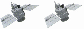
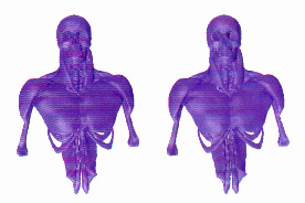
The following images were supplied by Renze and Oliver in their paper to show the testing which the surface decimation algorithm was subjected to. In each case, the image on the left is the original image, and the image on the right is that produced when the original image was decimated.
The distance-to-plane criterion is used to determine the candidate decimation vertices. Boundary vertices are degenerate topology are explicitly retained. The shaded figured were rendered using flat triangle shading.
The first image is a human pelvis, which was constructed from 3D anatomical data. The original image contains 34939 vertices, which was decimated by approximately 85 percent in the resulting image. Correspondingly, the approximately 70000 triangle faces in the initial image was reduced to about 10000 in the output.
The second image is an image of a satellite surface. The initial image contained 14112 vertices, of which about 21 percent were deleted in the final image. The number of triangle faces was reduced from approximately 25000 to about 19000. In this case, the CAD program which was used to create the initial image utilized an export format which clustered the majority of the vertices to define distinct features, such as sharp edges. This severely limits the number of vertices which can be reduced with the current decimation criteria while still preserving crispedge resolution.
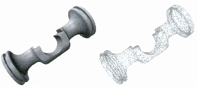
In the third image, the surface of a piston is illustrated. In this case, the resulting image is displayed as a wireframe in order to show how the vertices were preserved. The initial image, there were 15314 vertices, of which 76 percent were removed in the final image. Note that in the resulting image the vertices which remain seem to be concentrated in areas of high surface curvature, but gradual features tend to "fade out" as vertices are removed. This is based on the fact that the surface decimation algorithm is based on the current surface configuration, rather than the original.
In the fourth and final image, a human head and torso is depicted. The image was reconstructed from 3D anatomical data, as was the first image. The initial image contained 121547 vertices, of which about 66 percent were removed in the final image. Likewise, the number of triangular faces was reduced from about 243000 to about 80000.
This is where it starts to get more interesting, and more difficult (and more theoretical). The problem is that, given an unstructured surface definition, the problem of generating a valid volume tessellation of the interior domain is nontrivial. A set of points in three dimensions is always tetrahedralizable, except for the cases of a coincident, colinear, or coplanar vertex set.
The dual property of the 3D Voronoi diagram can be used to construct a colume tetrahedralization. However, unlike the planar counterpart, a nonconvex volume defined by a constrained face set isn't guaranteed to be tetrahedralizable. Renze and Oliver state the problem more formally: Determine if a 3D polyhedron can be decomposed into a set of nonoverlapping tetrahedra whose vertices are vertices of the polyhedron.
This problem was shown to be NP-complete by Ruppert and Seidel in their paper "On the Difficulty of Tetrahedralizing Three-Dimensional Nonconvex Polyhedra". An algorithm exists for tetrahedralizing a non-convex polyhedron by using Steiner points (points which are not vertices). This approach, while it works, goes against the goal of vertex-based volume decimation. In other words, adding points to tetrahedralize a constrained volume which was initially created by the removal of a vertex is counterproductive.
Instead, the hole created by the removal of a vertex is filled using a general unconstrained Delaunay tessellation algorithm. Topological sufficiency conditions indicate the inability to tetrahedralize a hole. If these conditions aren't satisfied, then the candidate decimation vertex can't be removed at the current decimation step. Instead, the vertex is queued at the end of the current decimation list for reconsideration later.
The volume decimation algorithm has less steps than the surface decimation algorithm. In this algorithm, given a volume tessellation, for each vertex v in the candidate decimation list, we do the following:
The local tessellation algorithm which was described earlier can be generalized to higher dimensions fairly easily. The general local tessellation algorithm presented by Renze in his dissertation "Unstructured Surface and Volume Decimation of Tessellated Domains" is similar to the planar tessellation algorithm, except that triangles are replaced with tetrahedra, and edges are replaced with triangular faces. In other words, triangles are replaced by n-simplices, and edges become (n-1)-simplices. The problem illustrated by the star-shaped polygon which caused failure in the planar decimation algorithm persists in this algorithm, with the additional complexity in identifying the number of valid insertion tetrahedra, and reconstructing the local boundary face loop.
The deletion of an interior vertex from a general surface topology requires that the size of the Valid stack be exactly two less than the original number of incident triangles. This topological sufficiency condition is derived from Euler's formula, and can't easily be extended to volume tetrahedralizations. Instead, Renze and Oliver developed a general local tessellation algorithm convergence mechanism.
If the Phase 1 classification produces an empry interior (n-1)-simplex set, then the hole region is convex or the candidate tessellation boundary is interpreted to be topologically inconsistent. "Convexity" can be tested by comparing the number of candidate n-simplices to the number of n-simplices placed on the Valid stack. The Phase 1 classification usually produces a non-empty interior (n-1)-simplex set for n>=3. The Phase 2 classification must result in an empty interior (n-1)-simplex set when it exits, in order to guarantee the topological sufficiency condition.
The deletion of a vertex v can result in an increase in the number of tetrahedra which tessellate the the original local boundary loop, when compared to the number of tetrahedra formarly incident at v. This means that a reduction in the number of vertices can result in an increase in the number of tetrahedra, although this doesn't usually happen.
The volume local tessellation can fail even in the event that the constrained geometry is untetrahedralizable. Look at the case of a unit cube which has an interior vertex v. Deleting v would create a degenerate condition for the unconstrained Delaunay tessellation algorithm, since more than four vertices would lie on the same circumsphere. The choice of the diagonal which determines the two faces on each side of the convex hull is not unique. Therefore, the existance of a nonempty interior (n-1)-simplex (face) set can be equated to inconsistant topology, if only a portion of the original boundary loop faces exist in the candidate volume tessellation. This local boundary loop ambiguity can be overcome with some additional logic.
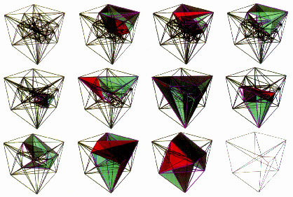
The figure below shows incremental stages of a unit cube volume decimation. Shaded regions show tetrahedra which were rejected during Phases 1 and 2 of the local tessellation classification algorithm for the current candidate decimation vertex. The initial volume tessellation consisted of 41 vertices and 189 tetrahedra. In the end approximately 70 percent of the original vertices were removed.
The following table shows the results of the decimation of nine different test geometries. The initial tessellations were generated using wither a Delaunay or Steiner tessellation technique. For example, the heat sink mesh included 7938 vertices and 32939 tetrahedra initially. The curved channel started with 23255 interior vertices, 117126 tetrahedra, and 7048 boundary vertices.
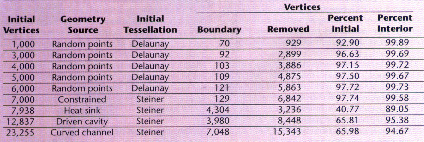
In all the cases nearly 90 percent of the original interior vertices were successfully removed. Note that the interior vertices in the Delaunay meshes are ultimately decimated more than 99 percent. This is significantly better than the Steiner tessellations in most cases, which may suggest that the Delaunay-based local tessellation algorithm is more efficient for decimating initial Delaunay tetrahedralizations then for initial Steiner volume tessellarions.
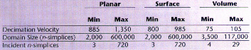
Now that we can decimate planar geometries, 3D surfaces, and volumes, we need a way to be able to determine just how good the performance of the decimation algorithms discussed above is. The decimation performance statistics given in Table 2 were produced by Renze and Oliver on a Silicon Graphics 150MHz R4400 machine with 128 MB of RAM.
The statistics reflect the average time which was required to identify a suitable interior vertex for decimation, produce a candidate local tessellation, classify the valid n-simplices that will preserve the local boundary loop topology and geometry, and finally update the connectivity for the current state.
The decimation velocity is defined to be the number of interior vertices removed from the tessellation per CPU second. The average decimation velocity remains relatively constant until the boundary limit is approached.
The number of incident triangles per candidate decimation vertex ranged from 3 to 720 for the planar and surface geometries tested. There was an upper bound observed of 10 to 15 triangles per local boundary loop.
The unstructured decimation algorithm described earlier can be used to greatly reduce the complexity of 2D and 3D triangulated meshes and 3D tetrahedral volumes. As shown by the development and test cases, it's robust, local, and n-dimensional. The authors conclude by making the following points:
While there are some problems with the algorithm, most of the time they'll never be seen. In general, decimation will allow us to reduce the complexity of an image, which in turns allows us to render that image with much greater speed.
Copyright © 1997 by John Pawasauskas