 .
This equation is a bit slow, due to the square root calculation, so like
Blinn, they recast it as a function in r**2 and R**2. By using an additional
condition (influence at R/2 = .5), the resulting function is
.
This equation is a bit slow, due to the square root calculation, so like
Blinn, they recast it as a function in r**2 and R**2. By using an additional
condition (influence at R/2 = .5), the resulting function is
 .
.
The typical method of modeling surfaces in computer graphics are using parametric equations to define points on the surface, which can then be connected to form polygonal meshes. This representation is very useful for performing transformations and computing surface normals. An alternative to parametric methods is the use of implicit representations, where the surface is defined as the zero contour of a function of 2 or 3 variables. Implicit representations have strengths in operations such as blending and metamorphosis, and have been becoming increasingly popular.
Metaballs, also known as blobby objects, are a type of implicit modeling technique. We can think of a metaball as a partical surrounded by a density field, where the density attributed to the particle (its influence) decreases with distance from the particle location. A surface is implied by taking an isosurface through this density field - the higher the isosurface value, the nearer it will be to the particle. The powerful aspect of metaballs is the way they can be combined. By simply summing the influences of each metaball on a given point, we can get very smooth blendings of the spherical influence fields (see images below).
The key to using metaballs is the definition of the equation for specifying the influence on an arbitrary point from an arbitrary particle. Blinn used exponentially decaying fields for each particle, with a Gaussian bump with height b and standard deviation a. If r is the distance from the particle to a location in the field, the influence of the particle is b*exp(-ar). For efficiency purposes, this was changed to the squared distance to avoid computing the squared root. The resulting density of an arbitrary location in the field is simply the summation of the contributions from all the particles.
Wyvill et. al. simplified the calculations somewhat by defining a cubic
polynomial based on the radius of influence for a particle and the distance
from the center of the particle to the field location in question. The key
is that the influence must be 1.0 when the distance r is 0.0, and 0.0 when
the distance is equal to the radius R of influence. A function which
satisfies these requirements is
.
This equation is a bit slow, due to the square root calculation, so like
Blinn, they recast it as a function in r**2 and R**2. By using an additional
condition (influence at R/2 = .5), the resulting function is
.
Once the field is generated, any scalar field visualization technique can be used to render it (Wyvill et. al. present a nice variation on the Marching Cubes algorithm in their paper which is very clever and efficient).
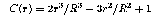
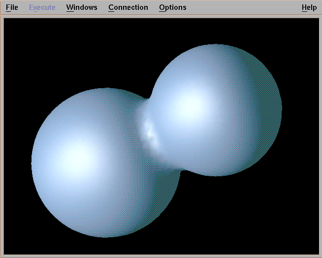
Here are some examples of two metaballs, one with a squared radius of 100 and the other with a squared radius of 125. All images are generated using IBM Data Explorer.
Two balls, threshold is .81.
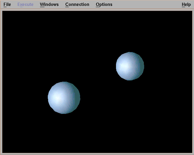
Two balls, threshold is .44.
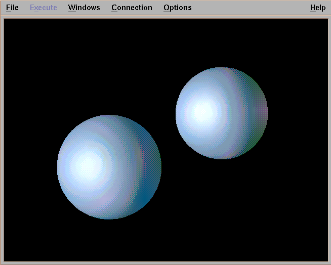
Two balls, threshold is .24.
Two balls, threshold is .11.
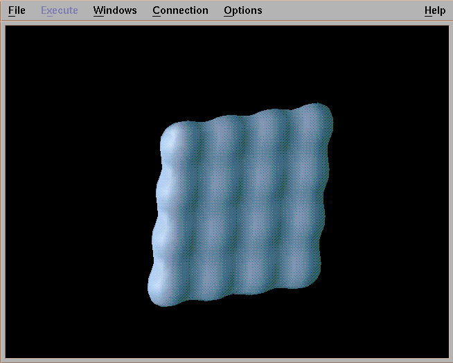
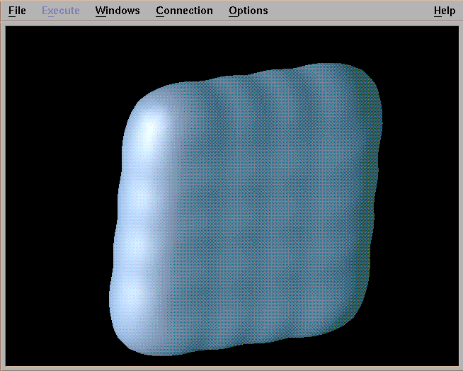
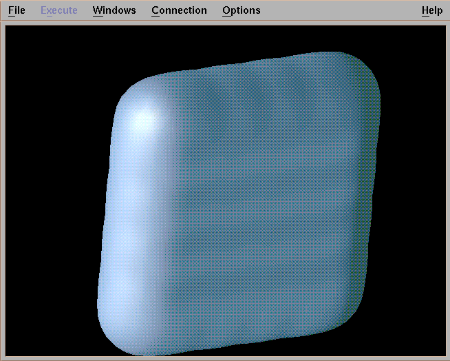
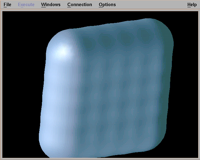
Here is a grid of metaballs, evenly spaced (5 apart) with a squared radius of 50.
25 balls, threshold is 1.66.
25 balls, threshold is .5.
25 balls, threshold is .26.
25 balls, threshold is .09.
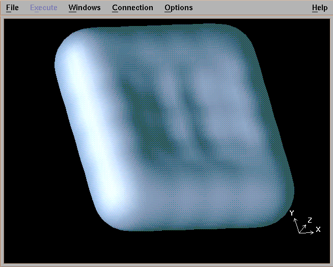
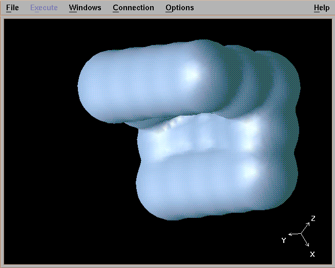
Now I change the squared radius of the inner balls to 30, to simulate a pad being pressed.
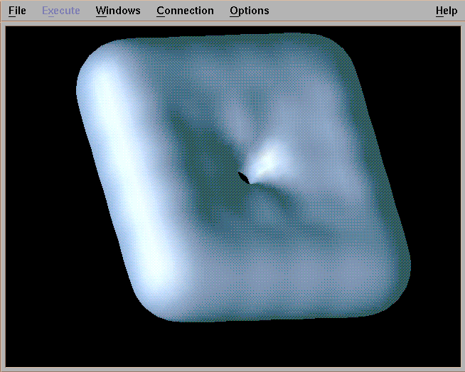
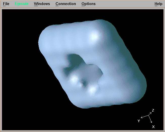
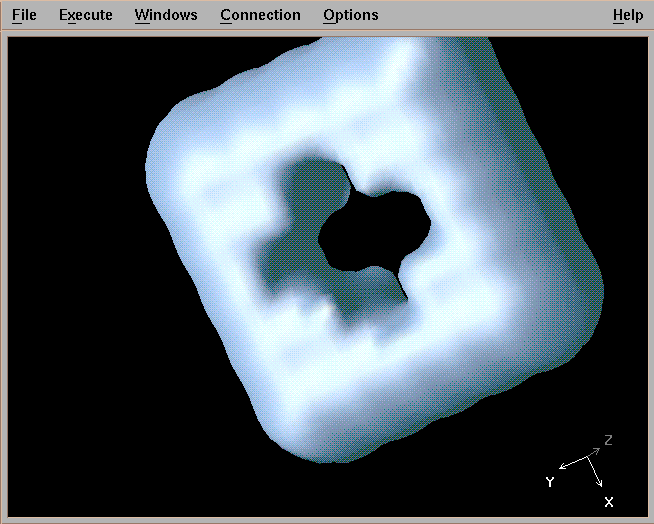
Now I eliminate the middle metaball to create a hole (threshold is .22).
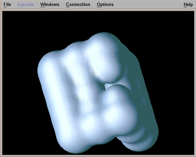
Now I change the positions of the balls to form a bend (threshold is .11).
Now I rotate the bent pad and lower the threshold to .05.
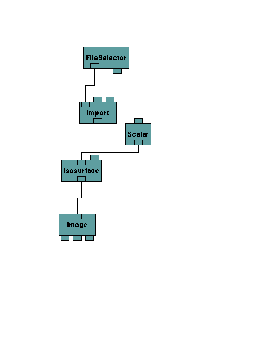
Here is the C code and Data Explorer Network that I used. The current maximum value on the slider which controls the isosurface value is set at 2. You may need to change this if you have very densely populated metaballs. However, most of the time you are interested in iso-values at or near zero.
The major problem I see in my implementation is that it is inefficient - basically I treat each metaball separately, and check the whole field to see if it has influence. A more efficient algorithm, especially for large fields, is to start at the metaball center and "grow" influence out until the radius is hit. This way you never examine empty parts of the field. Another optimization (if you have lots of balls with the same radius) is to create a 3-D template of influences and insert copies at locations in the field where you have metaballs. This would need to be adjusted in the case where balls do not lie exactly on grid points.
Basically, any monotonic function can be used to define a blob. Balls are simply the easiest to work with. Another extension which has been explored is the use of subtractive influences. My "pressed pad" would have looked much better, I think, if I had used subtractive balls rather than just reduce the influence of the inner balls. The math would be identical, up to the updating of the field. An extra flag for each metaball can tell you if you should add or subtract.
Below is my original pad, with 5 of the inner balls having a negative weight.
Here is another view. I'm not sure why some of the edges seem to have minor disturbances. Probably due to roundoff error.
J. Blinn, "A Generalization of Algebraic Surface Drawing", ACM Transactions on Graphics, Vol. 1, No. 3, pp. 235-256, July, 1982.
J. Menon, "An Introduction to Implicit Techniques", SIGGRAPH Course Notes on Implicit Surfaces for Geometric Modeling and Computer Graphics, 1996.
G. Wyvill, C. McPhetters, B. Wyvill, "Data Structure for Soft Objects", The Visual Computer, Vol. 2, pp. 227-234, 1986.
![[Return to CS563 '97 talks list]](/images/back.gif)