CS 110X Jan 27 2014

Lecture Path: 06
Back Next

Expected reading: pages 55-66.
Expected interaction: Math module
Clicker: Assessment

If I have seen further it is by standing on ye sholders of Giants.
Isaac Newton

1 Truth is ever to be found in simplicity, and not in the multiplicity and confusion of things

This lecture prepares you to generate graphical output in the form of mathematical plots. If you are a scientist you know the importance of data visualization. Many financial instruments can be best understood through similar graphical means. Over the course of this term, you will find it very useful to be able to generate plots of data. Let’s get started!

Python is so popular because of the many modules freely contributed to the standard Python environment.

Today I will introduce the pylab and numpy modules which contain an extensive set of functionality that you will find extremely useful. We would need seven weeks to simply cover all of the capabilities supported by these modules. You need to know about pylab and numpy because you should not try to "reinvent the wheel" when so many people have worked so hard to contribute this world-class numerical computation package.

pylab is simply part of the more comprehensive matplotlib project which contains countless tools that many scientists would find useful. You might find it inspiring to learn how other scientists are using Python to solve their problems.

Hundreds of examples for pylab are available, though it can seem daunting to read at first glance. In brief, if you have ever seen a type of graph appear in a scientific publication, you will likely find pylab sample code to show you how to recreate similar images.

So we’ll introduce numpy first and then pylab.

You want to determine the impact that steroids had on home run totals. You found statistics for the past 50 years that record the number of home runs hit by the top-ten players each year. You’d like to plot these numbers to see if anything "pops out" at you.

As you sit down to solve this problem, you should begin as follows:

# Assignment: Plot Home Run totals for evidence of steroid use # Author: George Heineman def plotHomeRunTotals(): # input # process # output

You are clearly laying out a strategy to solving the problem. Let’s first discuss how to get the input.

You will use a strategy that requires you know in advance how many items the user intends to enter. Since the computer cannot (yet) read your mind, you must prompt the user for this value, and then you can write a for loop to retrieve the proper information.

# Assignment: Plot Home Run totals for evidence of steroid use # Author: George Heineman def plotHomeRunTotals(): # input num = input("For how many years do you have data? ") for i in range(num): # collect data for each year, one at a time # process # output

See how you can immediately put the knowledge of for to use? Now you must consider what data you would like to collect for each year. For starters, assume that you have data that looks like this:

1950,47,37,36,34,32,32,32,31,31,31
1951,42,40,33,33,32,32,30,30,30,28
1952,37,37,32,32,31,30,29,29,28,25
1953,47,43,42,42,40,40,35,31,30,30
1954,49,42,41,41,40,40,35,32,29,27
1955,51,47,44,43,40,40,37,33,32,30
1956,52,43,38,38,37,36,36,35,32,32
1957,44,43,42,40,38,35,34,32,31,29
1958,47,42,41,39,38,35,35,31,31,30

The first row shows that the most number of home runs hit in 1950 was 47. This first row also shows that totals of the top-ten home run hitters; for example, in that same year the #2 home run hitter had 37 home runs, while the #3 home run hitter had 36.

Given this information, you decide that you are interested in storing for each year, the #1 total, the average of the top ten home run hitters, and the #10 total. You decide to plot these functions to see if you can spot any interesting trends.

1.1 Incrementally Constructing A List

Until now, all list variables were defined in one of two ways:

Coded in the program – for example:
temps = [30, 19, 22, 37, 45]
Input by the user all at once – for example, when the user input a comma-separated list of values, bracketed by "[" and "]" characters.
list = input("Enter numbers in the form [a, b, ..., z] ")

What you would like to do is incrementally append values to a list, to effectively create it one element at a time.

Here is how that would work.

The key point to the append function is how it is invoked. In English, you would say "I want to append the value of total to the highest list". In Python, you would say:

highest.append(total)

This is the first time you have seen the "dot" notation which uses the period (".") character. In this way you specify which list you want to modify.

Also note that append will only work if you actually have a list value to work with. For this reason, you first initialize highest to be the empty list []. Thereafter, in the for loop, you can safely append values to highest, increasing its size with each pass through the loop.

The above code is just a step towards our final solution. One good habit to follow is to try to always have something that executes, even if you only make small progress towards your overall goal.

If you execute the above program, you should see the following output:

>>> plotHomeRunTotals() For how many years do you have data? 5 Enter max number for year 0 47 Enter max number for year 1 42 Enter max number for year 2 37 Enter max number for year 3 47 Enter max number for year 4 49 [47, 42, 37, 47, 49]

You have successfully created a 5-element list by incrementally appending each successive value typed by the user. This is an incredibly useful skill to have, since it lets you operate flexibly without having to know in advance exactly how much data the user has available.

Now, this is one step towards solving your overall approach. Given this skill, you might extend the code as follows, asking the user to enter in all values in rather tedious fashion:

# Assignment: Plot Home Run totals for evidence of steroid use # Author: George Heineman def plotHomeRunTotals(): # input num = input("For how many years do you have data? ") highest = [] lowest = [] average = [] for i in range(num): total = input ("Enter max number for year " + str(i) + " ") highest.append(total) total = input ("Enter min number for year " + str(i) + " ") lowest.append(total) total = input ("Enter avg. number for year " + str(i) + " ") average.append(total) # process # output print (highest) print (lowest) print (average)

In fact, you are asking the user to compute the average, when that is certainly something your program should be able to do by itself!

What if you were to take advantage of your ability to enter in a list of values? Then the user would simply enter in a list of the top ten (or however many were available) home run totals for each year, and your program would compute the smallest, largest and average of that list.

Now that would be cool. And you can do it with a little help from numpy.

1.2 numpy Module

numpy is "an extension to the Python programming language, adding support for large, multi-dimensional arrays and matrices, along with a large library of high-level mathematical functions to operate on these arrays."

If you have ever heard of MATLAB (and how useful it is) then consider that numpy tries to give that power (for free!) to you.

numpy offers a dizzying range of functionalities. In this class we will focus on the statistics and mathematical functions.

The first new concept you have to learn is the import statement. Until you tell the Python interpreter about numpy, it won’t know what you are talking about. Kind of like how Trinity learned how to fly a helicopter in the Matrix.

As mentioned in class, when you run a Python module, you start with an empty Python shell. To access other functionality, you need to import the desired module as follows.

import numpy

In doing so, you make it possible to access numpy functionality. We will only scratch the surface of what numpy provides, but I will make sure to present in lecture every function that you might need to use for a homework assignment. I will never ask an exam question that depends upon knowledge of numpy (or pylab for that matter).

The three functions to start with are:

Maximum of a list – numpy.max(...)
Minimum of a list – numpy.min(...)
Average of a list – numpy.average(...)

With this knowledge in hand, you can now update your program as follows:

# Assignment: Plot Home Run totals for evidence of steroid use # Author: George Heineman import numpy def plotHomeRunTotals(): # input and process num = input("For how many years do you have data? ") highest = [] lowest = [] average = [] for i in range(num): list = input ("Enter home run totals for year " + str(i) + " as [h1, h2, ..., hn] ") highest.append(numpy.max(list)) lowest.append(numpy.min(list)) average.append(numpy.average(list)) # output print (highest) print (lowest) print (average)

Instead of having clearly identifiable input and process segments, this program processes the input as it is entered; this is a common strategy. To invoke one of the numpy functions, it is necessary to use the "." dot notation again, because these functions are defined by that module. Thus to invoke the max function defined in numpy, you must say numpy.max(...).

Now that you have accurate information, let’s show how to graphically visualize the data using pylab.

1.3 pylab Module

pylab provides extensive capability to plot data using a bewildering number of possibilities.

I will present the basic data-plotting mechanisms, and let you investigate on your own to discover the plots you might find interesting. The two most common plots are:

Smooth line-connected plot
Scatter plot of (x,y) values

For this assignment, I will show both types in action.

Once again, to enable this functionality you will need to import the pylab module. Here is a small example showing how it might prove useful.

>>> import pylab >>> xvalues = range(10) >>> yvalues = range(5, 15) >>> pylab.plot(xvalues, yvalues) [<matplotlib.lines.Line2D object at 0x044F80B0>] >>> pylab.show()

Once you press return on the last statement, a new window appears with the linear line drawn over x-coordinates in the range of 0 through-and-including 9, and y-coordinates in the range of 5 through-and-including 14.

The Python Shell is inactive, and it will not process any further input from the keyboard until you close the plot window. This window has a set of controls at the bottom that allow you to explore the plot, resizing or zooming in to individual regions; you can also save the image of the plot in a number of standard graphical formats.

You can integrate this logic into your program as follows:

# Assignment: Plot Home Run totals for evidence of steroid use # Author: George Heineman import numpy import pylab def plotHomeRunTotals(): # input and process num = input("For how many years do you have data? ") highest = [] lowest = [] average = [] for i in range(num): list = input ("Enter home run totals for year " + str(i) + " as [h1, h2, ..., hn] ") highest.append(numpy.max(list)) lowest.append(numpy.min(list)) average.append(numpy.average(list)) # output xvalues = range(num) pylab.plot(xvalues, highest) pylab.plot(xvalues, lowest) pylab.scatter(xvalues, average) pylab.show()

When run on a small set of data for the 1950-1959 decade, the following plot appears:

Figure 1: 1950-1959 Homerun Data

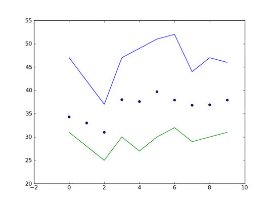
Note that this single plot is composed of three separate plot requests. The first two plot high and low values using lines; the last one produces a scatter plot of the average. All three use the same xvalues as the domain of the plot, and the y-axis reflects a range automatically computed from the values of the different plots.

The desired plot for data from 1950 through 2012 appears below.

Figure 2: 1950-2012 Homerun Data

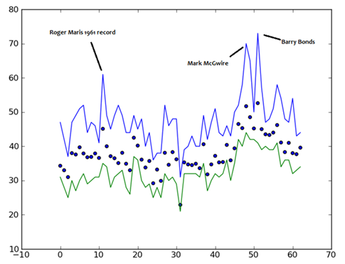
While by itself, this figure might not definitively prove anything, it certainly offers compelling evidence that during the late 1990s, the top ten home run hitters were achieving results that far exceeded the past performance of half a century.

This brief exercise is crude, but effective. You can consider enhancing the results by (a) considering more years; or (b) averaging data for more than 10 player per year.

1.4 Math module

The math module has extensive mathematical capabilities as well. For your homework2 you will likely find the following functions useful:

math.sin(x) – this returns the value of the Sine function.
math.factorial(n) – this returns the value of n! which is defined mathematically as n * (n-1) * (n-2) * ... 2 * 1.

These function only become available when you add the following statement to the beginning of your module:

import math

1.5 Debugging Challenge

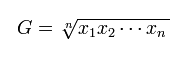
The following program is meant to compute the geometric mean for n values x1, x2, ... xn, entered by the user.

Figure 3: Formula for computing geometric mean

Can you find the defects?

Press To Reveal

# Assignment: Compute geometric mean # Author: George Heineman num = input ("How many values are you entering? ") product = () for i in range(1,num+1): val = input("Number ") product = product + val print ("Geometric mean " + str(product) ** 1/num)

Defects

1.6 Skills

In this lecture, you exercised the following skills:

DT-6: Know how to insert an element into a list
PM-2: Understand how to import a module
PM-7: Know about pylab module
PM-9: Know about numpy module
CS-9. Write definite for loop

1.7 Self Assessment

You need to become comfortable in devising input segments of your code that read a number of values as declared by the user. For example:

Type 1: Read in an entire list at a time.

A user wants to plot a number of (x,y) points in a scatter plot.

You should be able to write a Python module with a function makeScatterPlot() that takes the following as input and shows a plot window after the y-coordinates are entered.

>>> makeScatterPlot() Enter x-coords of the points as [x1, x2, ..., xn] [2, 7, 3, -1] Enter y-coords of the points as [y1, y2, ..., yn] [1, 2, 1, 2]

The resulting plot window should show the scatter plot with as many points as the user had entered.

Type 2: Read in a number, n, and then read that many values for processing.

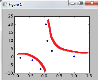
A user wants to sample a specific function, sin(x)*cos2(x)/x2 at a number of x-coordinates and plot it graphically.

>>> sampleFunction() Enter # of x-coordinates you would like to sample: 7 Enter x3: -0.13 Enter x2: -0.4 Enter x3: 0.05 Enter x3: 0.25 Enter x3: 0.1 Enter x6: 1 Enter x7: -0.8

The above code should draw a graph like the following. You should be able to do this now.

Figure 4: Sampling of Asymptotic function (red approximation added)

Draw arbitrary lines on a graph

Using pylab, you can issue multiple requests to plot and scatter; each time pylab will use a different color to draw the lines (or points) as appropriate.

Let’s say you just wanted to draw two horizontal lines. The following would work. And this idea should prove useful in tackling homework 2.

import pylab # Goal is to draw two lines. The first is from (0,10) to (100, 10) xvalues = [0, 100] h1Values = [10, 10] pylab.plot(xvalues, h1Values) # The second line is from (0, 40) to (100, 40). h2Values = [40, 40] pylab.plot(xvalues, h2Values) # domain of plot will be 0 through 100 pylab.xticks(xvalues) # range of plot will also be 0 through 100 yvalues = [0, 100] pylab.yticks(yvalues) # now show the graph pylab.show()

In the above code snippet, the call to yticks (and xticks) ensures that the y-axis (and x-axes) will use the scale from 0 to 100, enabling both horizontal lines to be easily visible.