Introduction
For realistic image synthesis we need shading models that adequately characterize the appearance of real-world surfaces. Shading models are often described as theoretical or empirical. Theoretical models are based on physical theory while empirical models are based purely on observation and measurement. At the heart of a shading model is the bidirectional reflectance distribution function (BRDF). It relates the incident light to the reflected light at a surface.
Finding the BRDF of a surface is the focus of much research. In this write-up we discuss a few of the techniques for measuring BRDFs and Wards shading model which fits a Gaussian distribution function to measured BRDF data.
BRDF
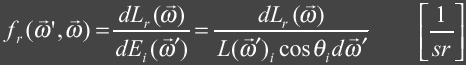
Measuring and Storing BRDFs
There are several techniques used to store BRDF measurements.
- Uniform and Non-uniform grid
This naive approach stores the sample points directly as a grid. To obtain the BRDF values between sample points neighboring sample points much be interpolated. One approach uses quadrilinear interpolation in which the 4 neighboring sample points are interpolated. This approach doesn't provide tangential continuity. Also, interpolation for non-uniform grids are more difficult. - Interpolating Spline
Fits an interpolating spline through the sample points. This approach provides smooth interpolation between sample points but often introduces high frequency noise due to oscillations in the curve. The noise shows up as artifacts in rendering. - B-Spline
Uses the sample points as control points for the spline. It provides smooth interpolation but the BRDF values at the sample points are not the original measured values. - Spherical Harmonics
This common technique represents BRDFs as a infinite sum of spherical harmonic basis functions. Large number of terms are needed to accurately represent general BRDFs and this technique also introduces high frequency noise. There are several techniques for noise reduction that are used. - Wavelets
Wavelets are basis functions that are good at representing signals that contain a great deal of high frequency signals in some areas while little in others. Wavelets are very attractive for storing BRDFs for this reason. Wavelets also provide good compression while introducing little error.
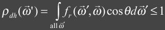
Traditional Gonioreflectometer
The figure below shows a traditional gonioreflectometer designed by Murray-Coleman and Smith.
 |
| Murray-Coleman and Smith Gonioreflectometer. ( Figure copied and modified from Ward[1] ) |
Imaging Gonioreflectometer
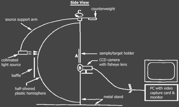
A small disadvantage with this device is that it can not capture reflectance at near grazing angles. It also is unable to measure polished surfaces with sharp specular peaks, due to the optical precision of the hemisphere. Technically the hemisphere should be a hemi-ellipsoid.
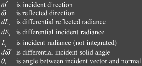
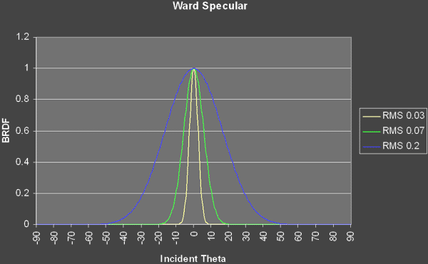
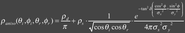
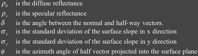
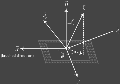
Ward Shading Model
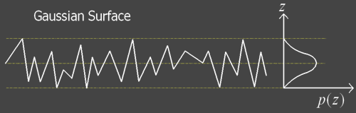
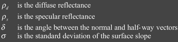
It is know in physics that rough surfaces tend to have Gaussian or normal distributions. It is the law of large numbers.
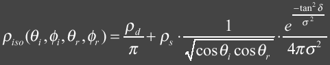
Ward first describes a mathematical model for isotropic surfaces.

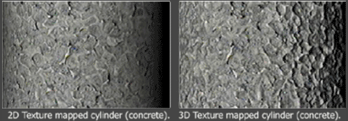
Bidirectional Texture Function
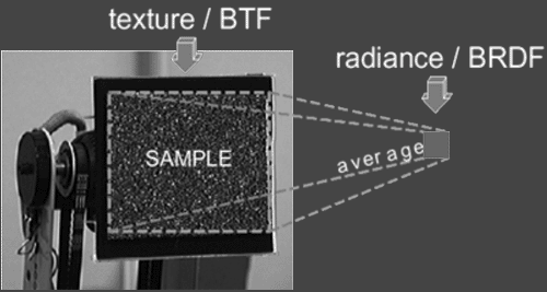
A BTF is a 6D function of 2D position, viewing and illumination angles. The BTF can be treated as a single texture map where the values of the texels are a 4D function of viewing and lighting directions. The u and v coordinates used to index the map is the position. Since the BTF consists of a large amount of images of the texture, computing the lookup value at (u,v) is expensive. It requires the lookup of all the samples that meet the criteria as specified by the lighting and viewing directions. To compute the final texture color these samples are then blended together. Overlapping regions of the samples are blended together.
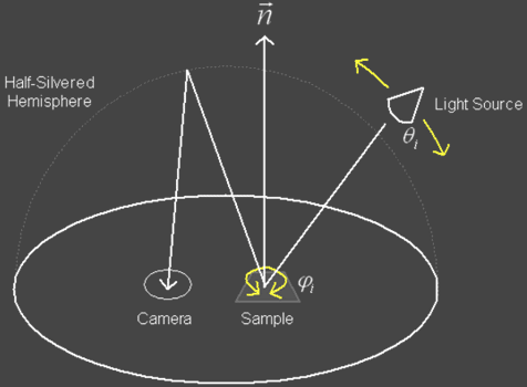
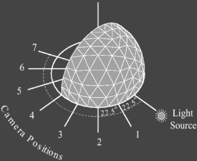
The device for generating a BTFs has a CCD color video camera, robot arm for orienting samples, light source with fresnel lens, spectrometer and PC for capturing the images. The fresnel lens is used to collimate the light. For BTF measurements the light source is fixed and the camera is positioned at seven locations. For each of the camera location images are captured for various orientations of the texture sample where it is both visible and illuminated. In the figure below the vertices of the hemisphere correspond to the direction of the sample's surface normal.
References
| [1] | Ward, Measuring and Modeling Anisotropic Relfection, Proc. ACM SIGGRAPH 1992 |
| [2] | White D.R. et al., Reflectometer for Measuring the Bidirectional Reflectance of Rough Surface, Applied Optics 37:16, 1998 |
| [3] | Dana et al, Reflectance and Texture of Real-World Surfaces, ACM Transactions of Graphics 18:1, 1999 |
| [4] | Tong et al., Synthesis of Bidirectional Texture Functions on Arbitrary Surfaces, ACM SIGGRAPH 2002 |
| [5] | Ke, A Method of Light Refletance, Masters Thesis, University of British Columbia, 1999 |
| [6] | DeYoung, Properties of Tabulated Bidirectional Reflectance Distribution Functions, Masters Thesis, University of British Columbia, 1996 |
| [7] | Glassner, Andrew Principles of Digital Image Synthesis, Morgan Kaufmann Publishers, Inc., San Fransico, 1995 |
| [8] | Shirley, Peter Fundamentals of Computer Graphics, A K Peters, Ltd, Massachusetts, 2002 |
| [9] | Hanrahan et al., Appearance Models for Computer Graphics and Vision, Stanford Lecture Notes at http://graphics.stanford.edu/courses/cs448c-00-fall/, 2000 |