|
Classical raytracing, an application of
geometric optics, point samples the incoming radiance from a scene by tracing
rays from the eye through the scene to the lights.
The images generated by an implementation of the classical raytracing
algorithm can look wonderful but also unrealistic and often times suffer from
severe aliasing problems. The
problem is that the algorithm severely undersamples the domains for the
integral equations that describe the complex optical interations of light.
Distribution raytracing, originally called
distributed raytracing, extends classical raytracing by incorporating
Monte Carlo
techniques. Instead of sampling
with one ray it distributes multiple rays to sample the integrals over the
pixel area, lens area, time, and the hemispheres for reflection and
refraction. This simple extension
is much more computationally expensive but as a point sampling process it is
necessary to render cool effects such as soft shadows, depth of field, motion
blur, glossy and translucent surfaces. Although
distribution raytracing is a huge improvement it does not solve the complete
problem.
|
|
|
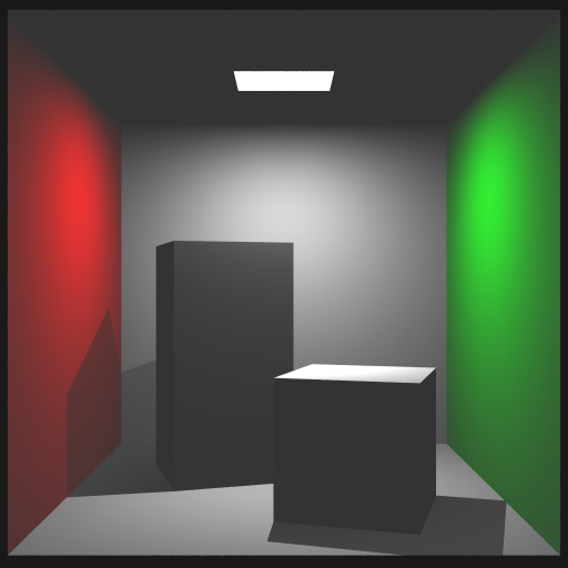
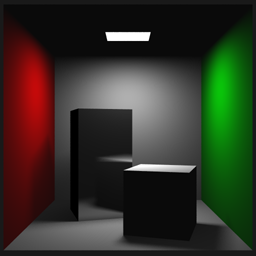
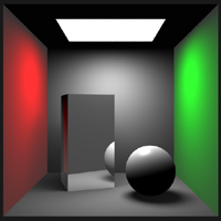
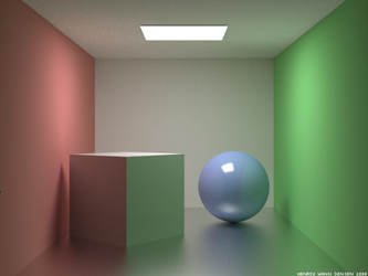
Cornell Box - Direct Lighting
16 samples were used per pixel, shadows and reflections. |
|
|
|
|
|
For realistic image synthesis we also need to
solve the rendering integrals for the light paths that account for global
illumination and caustics. However,
these integrals can be deeply nested and seemingly impossible to solve.
Using
Monte Carlo
techniques we have the facilities for approximating these integrals.
The basic idea behind
Monte Carlo
techniques is to approximate a function by randomly sampling it within some
domain. Hopefully, the samples give
some insight on what the functions look like.
Path tracing was developed as a solution to
the complete rendering equation and is heavily based on
Monte Carlo
techniques. It completely samples
the entire domain while distribution raytracing only samples portions of it.
Path tracing renders a scene by tracing rays from the eye back to the
light sources. Each of these ray
paths is a non-branching path where at each ray-surface interaction the new
direction for the path is determined probabilistically.
For the solution to converge to the correct result many rays are needed.
The main problem with path tracing is that the variance in the solution
shows up as noise. Fortunately,
there are ways to alleviate this noise such as using Photon Mapping to handle
caustics.
In the following sections I will discuss the
rendering equation, distribution raytracing, and will briefly touch upon path
tracing. This write-up reflects my
understanding of these topics and there may be errors.
If there are any please let me know.
|
|
|
The Rendering Equation
|
|
Introduced by James Kajiya in 1986, the rendering equation
describes the transport of light from one surface point to another as the sum
of emitted radiance and reflected radiance.
|
|
|
|
|
|
|
where:
|
|
|
|
|
|
|
Radiance tells us how much light energy is
arriving or leaving a surface in a particular direction within some time
frame. In a vacuum radiance is
constant along a line of sight which is an important property that makes
raytracing possible.
The term that is the most
interesting is the reflected radiance term, Lr, and can be described as the
following:
|
|
|
|
|
|
|
This integral takes into account all of the incoming light
and computes the reflected light. It takes into account all light paths
such as those that contribute to caustics and global illumination. The next several sections contains the details of this
integral.
|
|
|
Term
|
 |
: BRDF
|
|
|
|
|
|
|
|
The bidirectional reflectance distribution
function (BRDF) describes how a surface reflects light energy.
Reflectance is the fraction of incident light that is reflected.
The simplified form of the BRDF is a 4D function of incident and
outgoing directions. The BRDF is
given by the following ratio.
|
|
|
|
|
|
|
where:
|
|
|
|
|
|
|
For a BRDF to be physically plausible it must
follow the law of energy conservation and must obey the Helmholtz reciprocity
principle. Following the law of
energy conservation the BRDF should evaluate to a real number in the range
[0, 1]. To be more specific the
differential BRDF integrated over a hemisphere must be less then or equal to
one. This means we can not
reflect more light then we have received.
This can be expressed mathematically as follows:
|
|
|
|
|
|
|
This expression is also known as the directional
hemispherical reflectance and describes the total amount of incident light
energy that is reflected which must be less then or equal to 1. Helmholtz reciprocity principle
means that the sampling
incident and reflected directions of the BRDF can be switched and the result
will be the same.
|
|
|
|
|
|
|
Obtaining a BRDF for a material can be done in several ways.
One can obtain a BRDF through empirical measurements and then fit a
mathematical function to the data. Some
examples of these empirical models are the popular Lambert, Phong,
Blinn-Phong and Ward models. The
BRDF for a perfectly lambertian (diffuse) surface is just a constant as light
is equally reflected in all directions. Physically
based models can be developed analytically and are rooted in physics.
Examples of these are Cook-Torrance model and a model presented by
Kajiya in 1985 that handles anisotropic reflection.
|
|
|
Term
|
 |
: Incident Radiance
|
|
|
|
|
|
|
|
The function Li describes the incident radiance at x.
The function may be a deeply nested integral equation as incident
light may be indirectly reflected from other surfaces in the environment
including itself.
|
|
|
Term
|
 |
: Cosine Law
|
|
|
|
|
|
|
|
For this term we are taking the dot product of the incident direction and normal
to project the differential area subtended by the solid angle onto the base
of the hemisphere as seen by x. This term is necessary to account for
Lambertĺs cosine law. For a
better understanding we have the following:
|
|
|
|
|
|
|
Surface A is equally illuminated by surfaces B and C which both have the same
surface area. However, A can see
more of B then it does of C because the projected area of C onto A is smaller
then that of B.
|
|
|
Term
|
 |
: Differential Solid Angle
|
|
|
|
|
|
|
|
The differential solid angle is the differential
quantity of choice when integrating over a hemisphere.
The solid angle generalizes a range of directions through a
differential area on the hemisphere.
|
|
|
|
|
|
Solving the Rendering Equation
|
|
|
|
Two main approaches to solving the rendering equation are finite element
methods and point sampling techniques. For
the rest of this paper we will only discuss point sampling techniques using
Monte Carlo
methods.
|
|
|
Distribution Raytracing
|
|
|
|
Even before Kajiya formalized the rendering equation,
Cook et al recognized that rendering is just the process of solving a set of
nested integrals. Some examples
of these integrals are the integral over the pixel area, over the lens area,
over time, and over the hemispheres for reflection and transmission.
These integrals do not have an analytical solution that can be
computed in finite time, so instead we use
Monte Carlo
techniques to solve for them.
Basic idea behind
Monte Carlo
integration is to compute an average of random samples of the integrand f(x). The basic
Monte Carlo
integration can be described as:
|
|
|
|
|
|
|
where:
|
|
|
|
|
|
|
|
|
There are several forms of
Monte Carlo
integration techniques with varying random sampling strategies such as
importance sampling and stratified sampling.
Peter Shirley
shows that stratified sampling is often times far superior to importance
sampling. [1]
Stratified sampling is also easy to implement and no
prior knowledge of the signal is needed.
Basically, the domain is divided up into equal strata and then the
sub-domains are sampled by jittering samples about their centers.
|
|
|
|
|
|
|
At surface locations distributed raytracing does not completely integrate
over the entire domain, the hemisphere, but instead only over light sources
and about reflection and transmission rays.
Because of this distributed raytracing does not take into account all
light paths such as indirect illumination and caustic effects.
Never the less distributed raytracing is computationally expensive.
|
|
|
Sampling Pixels
|
|
Pixels have a finite area and represent a single color.
In classical raytracing we are sampling the incoming radiance from the
scene once per pixel.
|
|
|
|
|
|
|
From the start classical raytracing is grossly undersampling the scene.
Distributed raytracing extends classical raytracing to use stochastic
sampling, a Monte Carlo method, to approximate the integral over the area of
the pixel.
|
|
|
|
|
|
|
A common technique to approximate this nested integral is to use a jittered
grid, a form of stratified sampling, to sub-sample the pixel.
The basic idea is to divide the pixel area into a grid of equal size
cells or stata and the sample points are generated by jittering the center
point of each cell.
|
|
|
|
|
The pixel color is calculated by firing rays from the eye point through the
each of the jittered sample locations and then these samples are averaged.
|
|
click on images to enlarge
|
|

|

|

|
|
No Antialiasing |
4 samples per pixel |
16 samples per pixel |
|
|
|
Soft Shadows
|
|
In a basic raytracer implementation shadows are very sharp and typically this
is because point light sources are used.
In order to create soft shadows we need an area light source.
The figure below shows the anatomy of a shadow for both a point light
source and an area light source.
|
|
|
|
|
|
|
|
The umbra is the region where the light is entirely
occluded and the penumbra is the region where the light is partially
occluded.
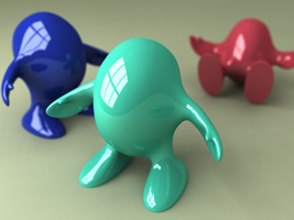
Soft shadows can be approximated in a standard
raytracer by just placing several point light source near each other where
each one has Nth the intensity of the base light they are approximating. Using
this technique sharp transitions occur in the penumbra because we are still
dealing with individual point light sources.
Here is an example where this technique is used.
|
|
|
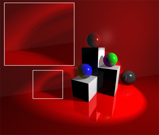 |
| RGBA Balls -
Notice the sharp transitions in the penumbra. |
|
|
|
|
Distributed raytracing resolves the problem by
stochastically sampling area light sources.
To implement this we can add a shadow factor to our rendering equation
that is a number between 0 and 1. A
shadow factor of 0 means we are completely occluded (umbra) or 1 if we are
completely unoccluded. A factor in
between 0 and 1 means we are partially occluded (penumbra).
The shadow factor is calculated for each light source by
generating a set of random sample points that are well distributed across the
surface of the light source and then distributing a set of shadow feeler rays to
these sample point locations.
|
|
|
|
|
|
|
Each shadow feeler ray, Si, either hits the light
source in which case it is assigned a value of 1 or it doesnĺt in which
case it is assigned a value of 0. To
calculate the lightĺs contribution we just take the average of the shadow
feelers and multiply it by the lightĺs intensity.
|
|
|
|
|
|
|
Generating the sample points over the area of the light source is done by
generating a jittered grid for n samples and then mapping the grid sample locations to a
set of locations on the surface of the light source.
The mapping for a square area light is straight forward.
|
|
click on images to enlarge
|
|

|

|
|
|
n=1 sample for shadows |
n=16 samples for shadows |
n=16 samples for shadows
Increased light size to increase the spread of the shadows. Also,
had to dim the light down. |
|
|
|
|
For other complex light types the mapping is not as simple.
However,
Peter Shirley
describes in an article called ôNonuniform random point sets via warpingö
for Graphics Gems III several warping transformations including that for
spheres, hemispheres and triangles. These transformations can be used
to map the jittered grid sample points to most complex light surfaces.
This of course assume the light radiates energy equally across its
surface.
|
|
|
Gloss
|
|
Glossy surfaces are specular surfaces that are somewhat rough.
Distribution raytracing tackles the problem by distributing a set of
reflection rays by randomly perturbing the ideal specular reflection ray.
The spread of the distribution determines the glossiness where a wider
distribution spread models a rougher surface.
|
|
|
|
|
|
|
To implement gloss you just need to setup a square that is perpendicular to
the specular reflection vector and then map a jittered grid of sampling
locations in which reflection rays are fired through.
The width of this square determines the glossiness of the surface.
In addition the ray contributions should be weighted using the BRDF or
the same specular weighting function used on the ideal specular reflection
rays.
|
|
|
|
|
|
|
Alone this technique can only model very shallow bumpy surfaces such as a
kitchen countertop where the distribution of the bumps is uniform.
However, we can incorporate a texture map that we look up into to
determine the pattern of glossiness where each texel in the map is a gloss
factor. The gloss map can be used
in addition to a bump map to model deeper groves.
|
|
|
|
|
|
|
Glossy floor using 16
secondary specular rays |
|
|
|
|
Translucency
|
|
Transluceny is implemented in a similar manner as gloss.
Once the bulk of the implementation is complete for gloss it is
straight forward to slightly modify it to include translucency.
The only difference is that instead of perturbing the ideal specular
reflection ray you are now perturbing the ideal specular transmission ray in
order to generate a set of secondary transmission rays.
A wider distribution of transmission rays will make the glass like
material appear rougher. Effects
such as frosted gloss can be achieved. For
a wider range of effects this technique can be mixed with translucent and
refraction maps.
|
|
|
Depth of Field
|
|
The depth of field is the distance that objects appear
in focus. It is necessary to
model a camera with a lens system to achieve depth of field effects.
For basic camera operation you need an opaque contain that contains a
single aperture (opening). This
aperture controls the amount of light that may strike the image or film.
Light passing through the aperture is the only light allowed to strike
the film. The amount of time that
the film is exposed to the light is controlled by a shutter.
In computer graphics the pinhole camera model is the
most popular. The film is
enclosed in a box containing a pinhole aperture.
Everything in the scene is sharply focused onto the image plane.
|
|
|
|
|
|
|
The pinhole which is infinitely small becomes the focal
point and the scene lies in front of it and is projected to the film which
lies behind the pinhole. In
computer graphics the typical setup is that the image and scene lies in front
of the focal point or point of projection.
Controlling the focal distance, the distance from the image plane to
the point of projection, or the image dimensions effects the field of view
but does not affect the focus of objects.
They will always appear in sharp focus.
A simple camera model for implementing depth of field is
the thin lens camera model. In
this model the camera lens is a double convex lens of negligible thickness.
This means that light passing through the lens is refracted on a
single plane called the principle plane instead of two refractions.
The lens has two focal points at equal distances in front and behind
the lens.
|
|
|
|
|
|
|
A phenomenon called the circle of confusion occurs when light from a single
point is focused through a lens onto an image as a circle.
The reason that this occurs is because the focal distance needed to
project the light as a single point is either in front or behind the image plane.
Remember light leaves a surface in all directions about the hemisphere
and thus the circle is formed because different parts of the lens are
focusing all light that it receives from the single surface point. In
the figure below light from the point on the focal plane is projected as a
circle on the image plane with distance C.
|
|
|
|
|
|
|
Given a focal length, f, and a
distance, i, which is the distance
from the pixel to the center of the lens, we can compute the depth of field
effects by first computing the distance, s,
from the center of the lens to a focal plane where all points will be in
focus. Using the thin-lens
approximation we can find s.
|
|
|
|
|
|
|
We now need to find a point P on the focal plane at
distance s that is in the line of sight from the center of the lens to the
pixel sample location. Once point
P is calculated we can generate a set of sample locations on the lens, again
using a jittered grid, from which we trace rays from to point P.
We can then average the contribution from these rays to find the color
at the pixel.
However, since we are also sub-sampling the pixel we
should pair samples from the pixels to samples on the lens.
To reduce alias artifacts we need to randomly pair the samples for
each pixel to locations on the lens.
Peter Shirley
discusses this in a tad more detail in his Realistic Raytracing book.
|
|
|
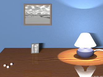
Zero Uno Toys - http://www.splutterfish.com |
|
|
|
Motion Blur
|
|
Motion blur occurs because the shutter allows the film
in the camera is exposed to light for a period of time.
While the shutter is opened any animation in the scene is captured on
a single piece of film. The
result is an image where objects in motion are blurred.
To implement this multiple rays from the pixel are fired
into the scene at different times and the contribution is averaged.
When taking into account depth of field, the computation can become
more costly. To reduce the
computation the samples in time can be paired with pixel and lens
samples. Then the rays traced
through these dimensions are then averaged for each pixel.
|
|
|
Path Tracing
|
|
Path tracing was introduced by Kajiya in the same paper that he formalized
the "The Rendering Equation". He developed path tracing as a
solution to the rendering the equation. It handles indirect lighting as
well as caustics. In a path tracer you are tracing a single path from
the eye back to the light source. Instead of distributing mulitple
secondary rays at each intersection, a single new ray path is chosen
probabilistically.
|
|
|
|
Kajiya points out that first generation rays as well as light source rays are
most important in terms of variance that they contribute to the pixel
integral. Secondary rays effect contribute less. When you are
only tracing a single path there needs to be a heuristic that tells the
algorithm where the important sampling directions are. Typically path
tracers incorporate an importance function that basically describe what parts
of the domain are important. Sample paths
are weighted according to their importance or contribution. We do not
need to solve for the entire domain as the overall result will not look much
different. For example, we only need an accurate solution of the
radiance equation for visible surfaces with significant contribution.
Importance needs to be propagated through the environment. If a surface
is important then any surfaces that contributes significantly to that surface
is also important.
|
|
|
|
One major problem with path tracing is that variance shows up as noise in the
final render. The main contributor to noise is caustics and can be
alleviated by using other techniques such as photon mapping.
|
|
|
|
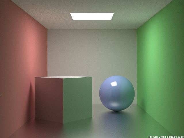
click to enlarge
|
|
|
|
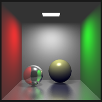
| 1000 samplers were used per
pixel. [Henrik Jensen] |
2000 samples per pixel. Jensen
states that render time was approximately 30 hours running on 30 SGI
workstations. [Henrik Jensen] |
|
|
|
References
|
| [1] |
Shirley,
Peter Realistic Raytracing A K Peters, Ltd. Massachusetts, 2000. |
| [2] |
Robert L. Cook, Thomas Porter, and Loren Carpenter.Distributed
Raytracing. Computer Graphics,
18(4):165-174, July 1984. ACM
Siggraph ĺ84 Conference Proceedings
|
| [3] |
James T. Kajiya. The Rendering
Equation. Computer
Graphics, 20(4):143-150, August 1986. ACM Siggraph ĺ86 Conference
Proceedings.
|
| [4] |
T. Whitted. An improved illumination model for shaded display.
CACM, 23(6):343-349, June 1980.
|
| [5] |
Glassner, Andrew An Introduction to Ray Tracing California: Academic Press Limited, San Diego, 1989 |
| [6] |
Glassner, Andrew Principles of Digital Image Synthesis Morgan Kaufmann Publishers, Inc., San Fransico, 1995
|
| [7] |
Shirley, Peter Fundamentals of Computer Graphics A K Peters, Ltd, Massachusetts, 2002
|
| [8] |
Jensen, Henrik W. Realistic Image Synthesis Using Photon Mapping. A K Peters, Ltd, Massachusetts, 2001
|
| [9] |
W. Heidrich, Ph. Slusallek, and H.-P. Seidel. An Image-based Model for Realistic Lens Systems in Interactive Computer
Graphics.
|
| [10] |
Giancoli, Douglas Physics for Scientist and Engineers. Prentice Hall, New Jersey, 1989
|
|