Sea Shells
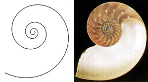
Many people admire the beauty of seashells. Some are fascinated by the various shapes and others are attracted to the different colors and unique patterns. However, while some people choose to collect seashells, others are motivated to construct their mathematical models. The purpose of modeling seashells is not simply to synthesize realistic images that can be used in computer generated scenes. It also allows us to gain a better understanding of the mechanism of shell formation. The logarithmic spiral, capturing the foundation of shell shape, was first described in 1638 by Descartes. By the beginning of the 20th century, it was observed in many organic forms.
Morphology is the branch of biology that "deals with the form and structure of organisms without consideration of function." David Raup is known as the pioneer of computer modeling of shell morphology. He published "Computers as aid in describing form in gastropod shells" all the way back in 1962. Raup said: “Successful simulation provides confirmation of the underlying models as valid descriptions of the actual biological situation; Unsuccessful simulation shows flaws in the postulated model and may suggest the changes that should be made in the model to correct the flaws.” Shell generating applets that follow Raup’s techniques can be found online.
There have been a number of advances in shell modeling techniques since Raup’s early work. In modern methods, the modeling of a shell surface starts with the construction of a logarithmic (equiangular) helico-spiral H. In a cylindrical coordinate system:
|
|
|
Parameter t, time, ranges from 0 at the apex of the shell to tmax at the opening. The first two equations represent a logarithmic spiral lying in the plane z = 0. The third equation stretches the spiral along the z-axis, thus contributing a helical component to its shape.
Distances r and z are exponential functions of the parameter t, and usually have the same base:
As a result, the generating helico-spiral is self-similar, with the center of similitude located at the origin of the coordinate system xyz. Given the initial values θ0, r0, and z0, a sequence of points on the helico-spiral can be computed incrementally using the formula:
While the angle of rotation θ increases in arithmetic progression with the step Δθ, the radius r forms a geometric progression with the scaling factor:
The vertical displacement z forms a geometric progression with the scaling factor:
In many shells, parameters λr and λz are the same. Below are some examples of shell shapes due primarily to different parameters of the helico-spiral.
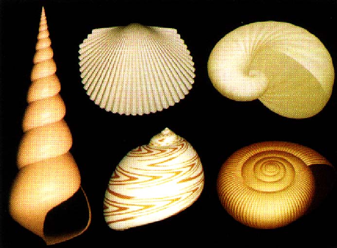
Turbinate shell (leftmost) z0=1.9, λ=1.007
Patelliform shell (top left) z0=0, λ=1.34
Spherical shell (bottom left) z0=1.5, λ=1.03
Tubular shell (top right) z0=0, λ=1.011
Diskoid shell (bottom right) z0=1.4, λ=1.014
The surface of the shell is determined by a generating curve C, sweeping along the helico-spiral H. The size of the curve C increases as it revolves around the shell axis. The shape of C determines the profile of the whorls and the shell opening. Generating curves are usually represented as Bézier curves.
Pigmentation patterns in shells are formed only along the growing edge of the shell. The shell forms as a result of deposition of new shell material which continually changes the position of the growing edge over time. Thus, the pattern on a shell can be viewed as a record of what has happened at the growing edge during the life span of a particular animal. Pigmentation patterns in seashells show an enormous amount of diversity. This diversity is due to the fact that a mollusk’s shell pattern lacks any selective influence. In a majority of cases, the animals live burrowed in the sand or are only active at night. Also, in many cases the pattern is invisible as long as the animal is alive, due to a covering layer. Consequently, there is no evolutionary pressure giving preference to specific shell patterns. Fowler et al use a class of reaction-diffusion models developed by Meinhardt and Klinger to simulate seashell pigmentation. Reaction-diffusion is not a single model, but the cornerstone of a whole spectrum of models. Fowler does not attempt to capture all possible shell pigmentation patterns in a single system of equations, but instead uses a different type of reaction-diffusion model to capture each class of pattern. The following will focus on the activator-substrate model, one type of reaction-diffusion model.
Catalyst - A substance, usually used in small amounts relative to the substrate, that modifies and increases the rate of a reaction without being consumed in the process. A substance that initiates or accelerates a chemical reaction.
Autocatalytic Reaction - A chemical reaction in which a product also functions as a catalyst. In such a reaction the observed rate of reaction is often found to increase with time from its initial value.
Substrate - The substance acted upon by a catalyst or enzyme. Often referred to as the reactant.
Activator - A substance, other than the catalyst or one of the substrates, that increases the rate of a catalyzed reaction without itself being consumed.
In simple terms, the activator-substrate model describes the complex interaction between the activator and the substrate. Pigmentation deposition is under the control of a substance, called the activator, which stimulates its own production through a positive feedback mechanism, or autocatalysis. In order for a pattern to be formed, a mechanism is also needed for suppressing the production of the activator in the neighborhood of the autocatalytic centers. This prevents the activator from spreading over the entire substrate. The pattern is formed as a result of the antagonistic interaction between short-range activation and long-range inhibition. The inhibitory effect results from the depletion of the substrate required to produce the activator. The interaction is described by the following equations:
The activator, with concentration a, diffuses along the x-axis at the rate Da and decays at the rate µ. Production of the activator is an autocatalytic process, proportional to a2 for small activator concentrations. This process can take place only in the presence of the substrate, and decreases its amount. ρ is the coefficient of proportionality and ρ0 represents a small base production of the activator needed to initiate the autocatalytic process. The autocatalysis can saturate at high activator concentrations, at the level controlled by the parameter κ. Similarly, the substrate, with concentration s, diffuses at the rate Ds and decays at the rate v. The substrate is produced at a constant rate s.
Initially the coefficient of proportionality (ρ) is subject to a small random fluctuation across the cells of the growing edge. The pattern that emerges after the initial transition is stable in time, but periodic in space. The periodicity is achieved by setting the range of inhibition to a fraction of the total length of the growing edge. The range of inhibition is determined by the diffusion and decay rates of the substrate. Concentrations of the activator, corresponding to fixed time intervals Δt, determine colors of cells (represented as pixels) in the consecutive columns or rims. Below is a stable pattern of stripes generated by the activator-substrate model.
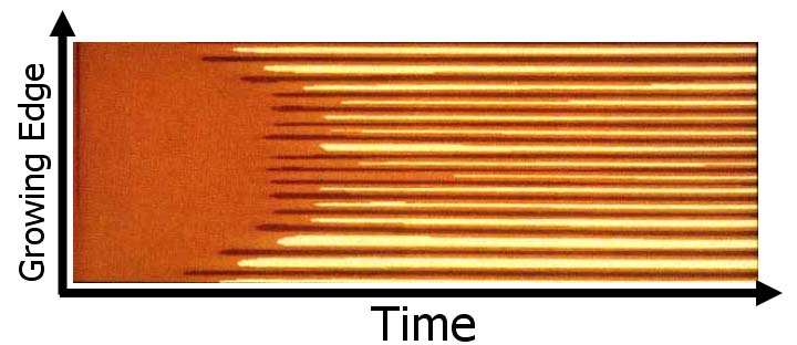

ρ =
0.01±2.5%
Da=0.002
µ = 0.01
ρ0 = 0.001
Ds=0.4
v = 0
σ = 0.015
κ = 0
The generation of stripes using the activator-substrate model is interesting from the theoretical perspective, since it illustrates the emergence of a pattern from an almost uniform initial distribution of substances. The fact that patterns develop in a homogeneous medium is what motivated the original studies of the reaction-diffusion models.
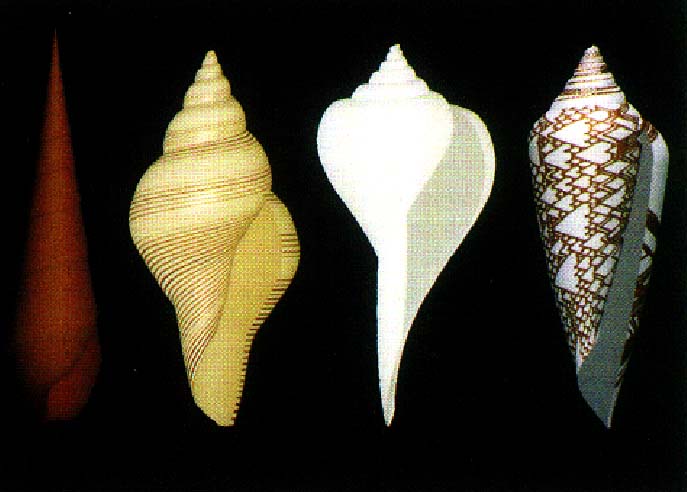
In order to generate lines of undulating shapes, we assume that the activator-substrate model is regulated by an external factor. This modulates the substrate production σ according to a periodic function of cell position. In regions with higher σ, oscillations are faster than is regions with lower σ concentrations.
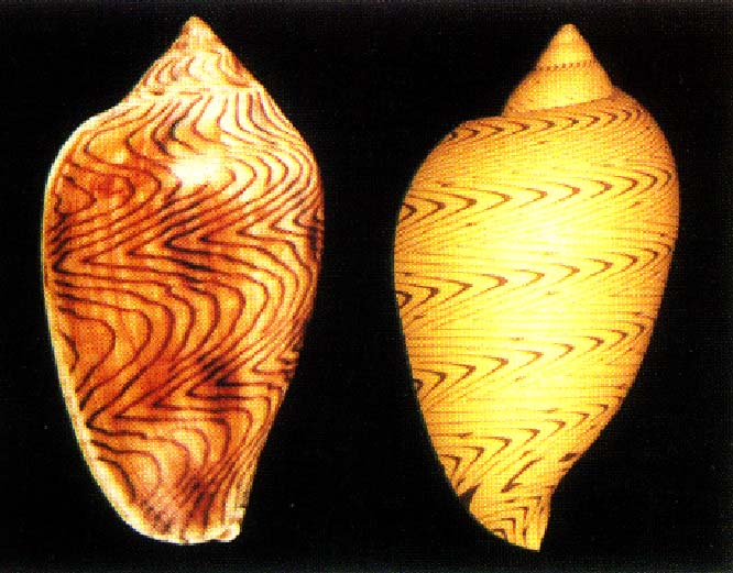
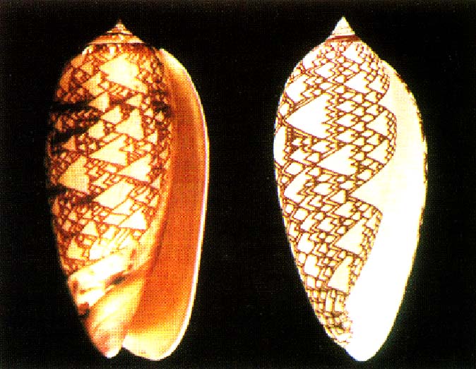
Photograph on the left. Rendered image on the right.
[1] D. Fowler, H. Meinhardt, and P. Prusinkiew, Modeling Seashells, (Proc. ACM SIGGRAPH '92, pages 379-388)
[2] D. Raup, “Computer as aid in describing form in gastropod shells,” Science (138: 150-152, 1962)
[3] A. Witkin and M. Hass, “Reaction-diffusion textures,” Computer Graphics (25.4:299-308, 1991)
[4] C. Pickover, “A short recipe for seashell synthesis,” IEEE Computer Graphics and Applications (9.6:8-11, 1989)