Bi-Directional Reflectance Distribution Functions

by Chuck Moidel

Introduction

The goal of realistic rendering is to create computer generated pictures of synthetic scenes almost indistinguishable from photographs of real environments. To achieve this goal we must simulate the behavior of light, from the source, interacting with the scene, and finally reaching the camera. Such a simulation involves global illumination and local illumination algorithms. Global illumination algorithms try to collect the contributions of all parts of the environment which are illuminating a given point of the scene, while local illumination algorithms try to compute the transformation that occurs at this point between incoming and outgoing light [2]. The topics contained in this paper, specifically BRDFs, fall under local illumination models or LIMs.

A BRDF, bi-directional reflectance distribution function, is a tool for describing the distribution of reflected light at a surface. Given an incoming light ray at a point on a surface, the BRDF is used to calculate how much of that light ray will be reflected in a particular outgoing direction. Specifically, the BRDF is an approximation of the BSSRDF, bi-directional sub-surface scattering reflectance distribution function. The BRDF ignores sub-surface scattering and assumes that the light striking the surface at some point will be reflected from that same point.

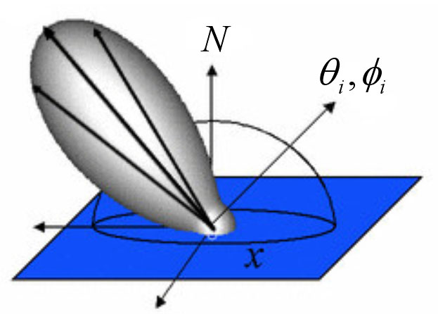
Figure 1: This is the BRDF output response for a light ray with fixed input direction q,f

Solid Angles

In order to understand the definition of a BRDF it is important to understand some fundamentals. In radiometry, when considering a point on the surface, many of the measurements are taken with respect to the unit hemisphere surrounding that point. The solid angle is used to refer to some small surface area on the hemisphere. A solid angle is approximated in terms of the area on a sphere intercepted by a cone whose apex is at the sphere’s center. A steradian (sr) is the solid angle of a cone that intercepts an area equal to the square of the sphere’s radius [6]. There are therefore 2p steradians in a unit hemisphere.

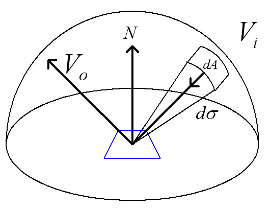
Figure 2: The image shows the steradians dσ that measure some surface patch dA

Irradiance and Radiance

Irradiance is the measure of how much light hits a point from all incoming directions. Irradiance, E_i, is the rate of incident or incoming energy at a surface point per unit surface area. The units of irradiance are watts per meter squared, W/m². Incident light contributes to irradiance, E_i, while reflected light, or exitant light, contributes to radiant exitance, E_o. Whereas irradiance describes how much light is arriving at a point from all directions, radiance describes how much light is arriving at a point from a specific direction. Incoming radiance, L_i, is also referred to as field radiance and outgoing radiance, L_o, is also referred to as surface radiance or scene radiance. The units of radiance are watts per steradian meters squared or W/(m² × sr). We can compute the irradiance at a point on the surface by summing up the incoming radiance from every direction on the hemisphere that surrounds that point.

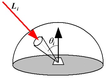
Figure 3: Definition of irradiance

BRDF Definition and the Transport Equation

The BRDF, referred to as R_l, is defined as the outgoing radiance divided by the irradiance. The units of the BRDF are therefore inverse steradians. A BRDF describes the relation between the incoming and outgoing radiances at a given point P on the surface. This is because the BRDF is a function of irradiance and the irradiance takes into account all incoming radiances. Because the BRDF is a ratio, the values are independent of the strength and geometry of the light source. This is very important, because it allows BRDF values calculated or measured on a material in one set of lighting conditions to be applied to that material under any lighting conditions.

Figure 4: Definition of BRDF

Figure 5: Transport Equation or Rendering Equation

Using the Transport Equation, one can determine the outgoing radiance at a point P from the BRDF and the irradiance. In figure 5, L_o(P,V_o) refers to the reflected radiance leaving the point P in direction V_out. R_λ(P,V_o,V_in) defines the BRDF of the surface at P from V_out and V_in. L_i(P,-V_i) describes the incident radiance reaching point P from direction –V_in. N dot V_i describes the cosine of the angle between vector N and V_in. The last part, dσ, describes the differential solid angle surrounding the direction V_in.

Figure 6: Angles and vectors used to represent the BRDF (click to zoom)

BRDF Constraints

All proper physical based BRDFs obey two constraints: the Helmholtz Reciprocity Rule and the Energy Conservation Law. Most empirical models, such as the Phong lighting model, overlook these rules. The Helmholtz Reciprocity rule, which results directly from the physics of light, states that the BRDF R_λ is symmetric relative to V_in and V_out [2].

Figure 7: The Helmholtz Reciprocity Rule

Figure 8: The Energy Conservation Law

The energy conservation law also results directly from the physics of light and serves to normalize the BRDF R_λ. It states that no more than 100% of the incident radiance can be reflected at any one point. This can be seen from the equation in figure 8 because the BRDF R_λ is the ratio of outgoing radiance divided by the irradiance and the outgoing radiance can never be greater than the irradiance. This is because the irradiance already takes into account all incoming radiance at a point and there can not be more light leaving from a point than there is light arriving at that point.

Acquiring BRDFs

BRDFs can be computed from analytical models or captured using sensitive instruments [1]. For example, He’s theoretical BRDF model considers Fresnel reflections, subsurface scattering, surface micro-geometry, and self-shadowing. The surface micro-geometry model treats the surface as a collection of micro-facets, considered perfect reflectors, with random sizes and orientations. The self-shadowing model tries to account for the fact that light can interreflect off of several micro-facets or be occluded completely. He’s model can accurately predict specular reflections at grazing angles and accurately calculates physical phenomena resulting from rough surfaces.

Instead of using a theoretical model, Westin uses simulation based methods to determine the BRDFs of complex surfaces. Westin starts with a geometric model representing the microgeometry of a small surface patch. This patch is then used as input to a ray tracer which itself uses a known BRDF to compute reflections from incident light. The algorithm computes the average amount of light reflected into each outgoing angle from each incoming angle. Whereas He’s model assumes the surface consists of randomly oriented microfacets and therefore cannot represent anisotropic surfaces, Westin’s method can model any kind of complex surface without restriction.

The device used to physically measure a BRDF is called a gonioreflectometer. Since BRDFs are a function of four dimensions, physically measuring them is very challenging. There are often problems with consistency of the light source, camera stability, variations in surface geometry, and interreflections. This can lead to huge variations in results measured from identical samples [1]. Because of these problems, theoretical or simulation models are preferred.

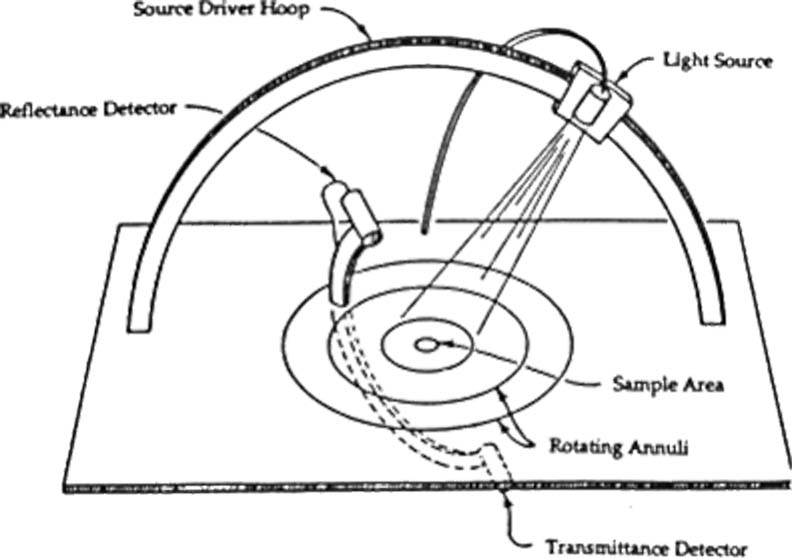
Figure 9: Gonioreflectometer (click to zoom)

Representing BRDFs

Sophisticated and elaborate BRDFs often take into account incoming and outgoing angle, wavelength, polarization, position, and time. These are too many variables for computer graphics, since this can lead to lengthy computation. More simple BRDFs consider ray optics rather than wave optics when computing light transport. Ray optics treats light as non-interacting straight rays each carrying a certain amount of energy [2]. Ray optics simplifies the notation and expressions of equations by neglecting wavelength. Because wavelength is neglected, so are the effects of interference, diffraction, and polarization that result from light wave interaction.

Computer graphics requires BRDF representations that are accurate, have high angular resolution, and cover all possible angles of incidence and reflection. Traditionally, computer graphics systems either relied on analytical models or had to store enormous amounts of data to represent even simple BRDFs. The most simple BRDF representation, called Scatterometry, stores samples of the BRDF on a regular four dimensional grid and interpolates between them. Using this method, the interpolated data is likely to be noisy and yield unsatisfactory results. Also, there are usually missing data points near the grazing and backscatter angles which causes more problems. In addition to these problems, storing a complete BRDF sufficiently densely for computer graphics needs is likely to require millions of data points [4].

Given the size and high dimensionality of BRDFs, many techniques have been developed to store and compute them efficiently. Modern techniques for storing BRDFs are: fitting to analytical models, using spline patches, using spherical harmonics, using spherical wavelets, and using Zernike polynomials. Also, a change of variables with one of the previously mentioned techniques can lead to a more efficient representation. Spline patches solve the problems of simple interpolation by smoothing the data. While this leads to less noise, it still requires a very large amount of storage to represent the BRDF.

Using spherical harmonics to represent the BRDF is another approach that is more efficient than simple scatterometry or spline patches. Spherical harmonics are the spherical analogues of sines and cosines and are localized in the frequency domain. Each part of the signal is known as a basis function and the sum of all of the basis functions reproduces the original signal exactly. Because there may be an infinite number of basis functions required to exactly reproduce the desired BRDF, usually only a subset of these basis functions are used. However, to accurately represent the BRDF for computer graphics needs, the subset may still need to contain a very large number of basis functions for either spherical harmonics or Zernike polynomials. Using too few basis functions can result in “ringing” cased by sharp edges in frequency space and using too many basis functions is computationally very expensive.

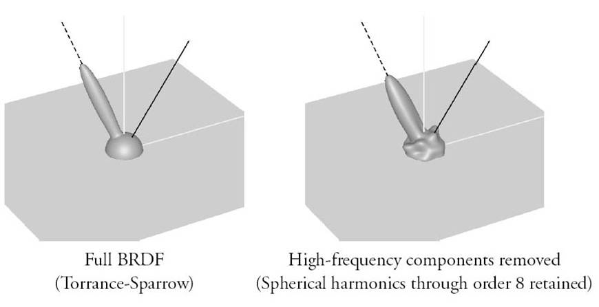
Figure 10: Using too few basis functions (click to zoom)

Even though spherical harmonics are an efficient way to represent a BRDF, there are still more efficient techniques. Because we are representing a BRDF, we are only interested in a hemisphere and not an entire sphere. Using a basis of spherical harmonics treats functions on a hemisphere as a special case of functions on a sphere. An alternative is to use basis function on a disk and then map those function onto a hemisphere. Using Zernike polynomials, which form an orthonormal basis of functions on the unit disk, a representation can be optimized for the hemisphere. Rusinkiewicz discovered that a change of variables can transform BRDFs such that they can be represented more efficiently using basis functions. This causes some features of common BRDFs to lie along new coordinate axes and reduces the number of basis functions required to accurately reproduce the BRDF.

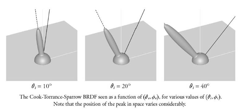
Figure 11: BRDF representation using conventional variables (click to zoom)

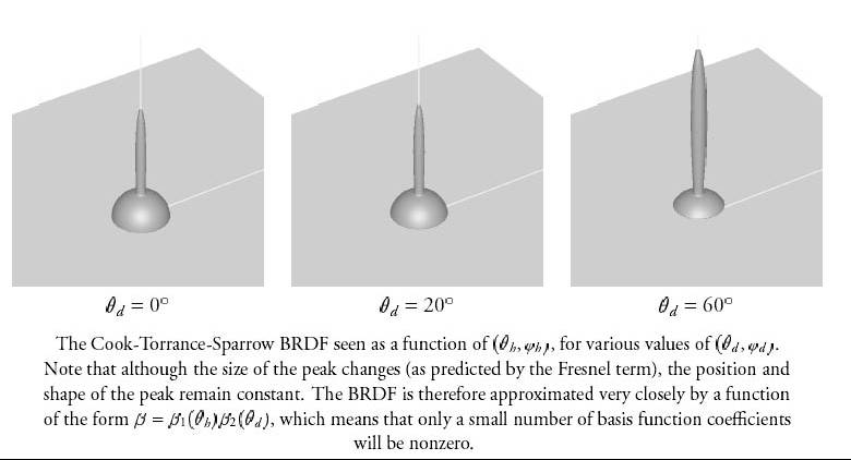
Figure 12: BRDF representation using change of variables (click to zoom)

References

[1] Szymon Rusinkiewicz, A Survey of BRDF Representation for Computer Graphics (Paper for CS 348C at Stanford U., Winter 1997) (online)

[2] Christophe Schlick, “A Survey of Shading and Reflectance Models,” Computer Graphics Forum 13 (June 1994) 2:121-132 (online) (online)

[3] Peter Shirley et al., A Practitioners' Assessment of Light Reflection Models (Pacific Graphics, 1997) (online)

[4] Szymon Rusinkiewicz, A New Change of Variables for Efficient BRDF Representation (Eurographics Rendering Workshop, 1998) (online)

[5] Peter Shirley, Fundamentals of Computer Graphics (Massachusetts: A K Peters Ltd, 2002) (info)