CS 563 Advanced
Topics in
Computer Graphics
View Interpolation and Image Warping
By
(No consent was allowed for the information or pictures used within)
(Link to Slides of this Paper)
Introduction:
So where to start? Well first let me give you some slight background information on Image Based Rendering (herein IBR). IBR is the generation of a 3D scene from 2D objects. The input for such a process is composed of photometric observations (or pictures). This field of IBR is actually a mixture of many. It includes photogrammetry, vision and computer graphics. All of these fields in parts add to the field of IBR.
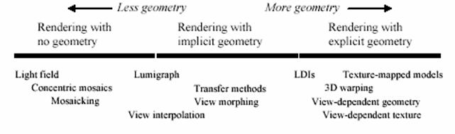
Some of the current uses of IBR are in texture mapping and environment mapping. Texture mapping will map a 2D image to a 3D object to create the idea of a more detail 3D image at a lower cost than actually trying to render the 3D object at that complexity level. Environment mapping is when an object will reflect the environment around it, be it a 2D image or another object. These techniques provide very realistic surface models and can save much on the processing cost when compared to creating a complex 3D objects these images represent. Some of the uses of having such low cost rendering are things that require real time response like video games or virtual reality. The results that are displayed from IBR are usually hard to judge because there is no set standard for them. Of course there is always the one test of how it looks to you and other viewers. The human eye is one of the best judges since it find imperfection so quickly. The figure below shows the level of geometry that is used to render images using different techniques. The area this paper will concentrate mostly on is the View interpolation.
Interpolation:
The topic of the first paper I read
and the one that covers the largest portion of my paper is “View
Interpolation”. One use for TBR is in
real time environments like games and virtual reality. A useful method to accomplish this task is
using a large number of views of an environment from closely space view points. This can be used for virtual tours or
something like a flight simulator. The
typical approach has the computer rendering the scene from each different view
point. This approach is both
computationally expense (usually requiring specialized graphics hardware) and
the rendering speed is dependent on the scene complexity which can create lags
in the rendering.
Some past approaches to this problem
have used a pre-process to compute the subset of a scene that is viewable from
a specific viewing region. This approach
has problems in that there may be viewing regions were all objects are
visible. Another uses pre-computed
environment maps with Z-buffered images.
The environment maps are stored in a structured way and an image from a
new view point can be generated using the adjacent environment maps. The advantage of this technique is that the
rendering speed is proportional to the environment map resolutions and not the
scene complexity, but this method does require Z-buffer hardware to render a
relatively large number of polygons interactively.
The technique I will talk about in my paper
presents a fast method to generate intermediate images from images store at
nearby view points. Similar to the
second technique I talked about above in that this techniques rendering time is
independent of the scenes complexity. Unlike
that technique the one discussed here uses image morphing of the adjacent
images to create and in-between image from a viewpoint. Image morphing is the interpolation of
different texture maps and shapes into one.
The morphing uses pre-computed correspondence maps which allow it to run
efficiently and at interactive rates.
This method depends highly of the fact that the images used are taken
from closely spaced viewpoints. Also it
used the cameras position and orientation, and the range data of the image to
determine a pixel-by-pixel correspondence.
This method can be used with either synthetic or real images. It wants to capture the ranges data and camera transformations to allow for pixel to pixel correspondence between images. This data can be gathered easily if the image is synthetic and for natural images a ranging camera can be used along with photogrammetry to obtain the information. Though it was only tested with synthetic images, the method can be applied to natural images. Of course this paper/experiment was conducted in ’93 so by now natural images may have been tested. Also the interpolation of the images only accurately supports view independent shading. Reflection mapping and Phong specular reflection could be used with separate maps but they are discussed, but only diffuse reflection and texture mapping are discussed here.
This morphing method can be used to interpolate many different parameters, such as the camera position and orientation, viewing angle, direction of view and the hierarchical object transformation. The modeling and viewing transformations can be combined to compute the correspondence mapping between two images. The images that are used can be set up in a graph structure for easy access. The nodes of the graph would be the images and each arc represents a correspondence mapping between images.
Visibility Morphing:
There are two steps to the image
morphing process the first is finding the correspondence between the images,
this is the most difficult step. Typically
this is done by an animator who would determine specific points that correspond
in the different images and let an algorithm determine the rest. The second step is two interpolate the shape
of each image towards each other, depending on the view to be rendered and to
blend the pixel values of the two warped images by the same 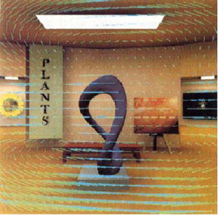 coefficients.
This method uses the camera transformations and the image range data to automatically calculate the correspondence between two or more images. The correspondence is a form of forward mapping. The mapping describes the pixel by pixel map from the source image to the destination image. This technique is bi-directional allowing either image to act as the source and the other the destination. Pixels are mapped to their location on the destination image. If the pixel maps to the same pixel in the interpolated image the Z-coordinates are compared to figure out which is visible. Cross dissolving of pixels may be necessary if the image colors are not view – independent. This method is made even more efficient by the use of a quad-tree compression algorithm. What this will do is group pixels that are adjacent to each other and are similar in both images. These will be compressed and moved together.
As we all know when you move a camera in one direction the scene you’re looking at moves in the other. When moving from one image to the other there is a change in position for the pixels because of this. Since we know the pixel’s coordinates and the scenes camera coordinates we are able to calculate this movement. This movement is stored as a 3D spatial offset vector for each of the pixels, and is stored in the morph map. This mapping is many to one since many pixels from the first image can move to one pixel of the second image. The smaller the change in the offset vectors is the more accurate the interpolation of the new scene will be. Larger changes are harder to deal with since the information for any space that becomes visible from the new position that isn’t covered in either of the samples will have to be interpolated over. The figure to the right shows the offset vectors for the camera motion sampled at 20 pixel intervals.
Overlaps and Holes
Overlaps occur due to image contraction. This is when many pixels of one image are moved to one pixel of the other. Take an image that turns so that one side is closer to you and the other is further away. Perception will show the side closer to you to be larger and the side that is further away to be smaller. Samples that are on the far side of the image will contract and the samples near to you will expand. The contraction causes samples to overlap in target pixels.
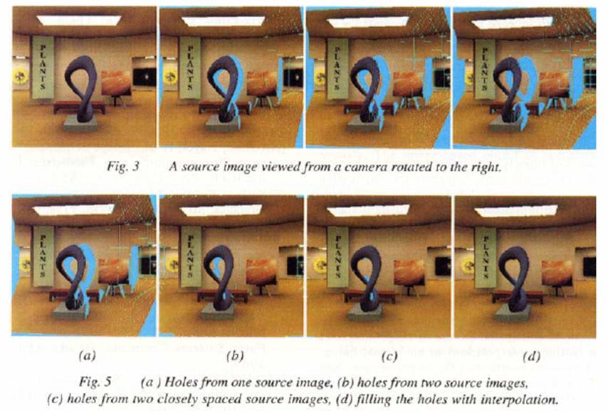
Holes can occur when mapping the
source to the destination image. An
example of this is shown the image below (in the figure labeled figure 3). The cyan regions in figure 3 represent the
holes. This color is pre-chosen and set
as the background so any holes that appear are noticed easily. In the case of figure 3 you can see the
camera is moved to the right and the image to the left creating spots that
aren’t covered by a pixel from one of the sampled images. When a square pixel is mapped to the
destination image it’s 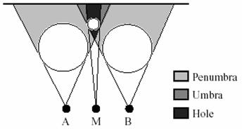 mapped
as a quadrilateral. To solve the problem
of the holes we can interpolate the four corners of a pixel instead of its
center. Then the holes can be eliminated
by filling and filtering.
mapped
as a quadrilateral. To solve the problem
of the holes we can interpolate the four corners of a pixel instead of its
center. Then the holes can be eliminated
by filling and filtering.
Another solution to eliminate the holes that is more efficient is to interpolate the adjacent pixels’ colors, or offset vectors. Knowing the background color allows us to determine where the holes are and the surrounding pixels that can be used to interpolate color values for the pixels where the holes are found. The offset vector can be interpolated for the pixels in the hole and used to index back to the source image to obtain a new color for each pixel. Or using multiple images to interpolate the new image can alleviate the problem of holes but not eliminate it. The last possibility for holes comes from a spot that is visible in the image to be interpolated but not visible by the view points of the images that are used to interpolate the new image. This is shown in the picture to the right. A solution for this would be to use multiple images to minimize the umbra region (as shown in the picture).
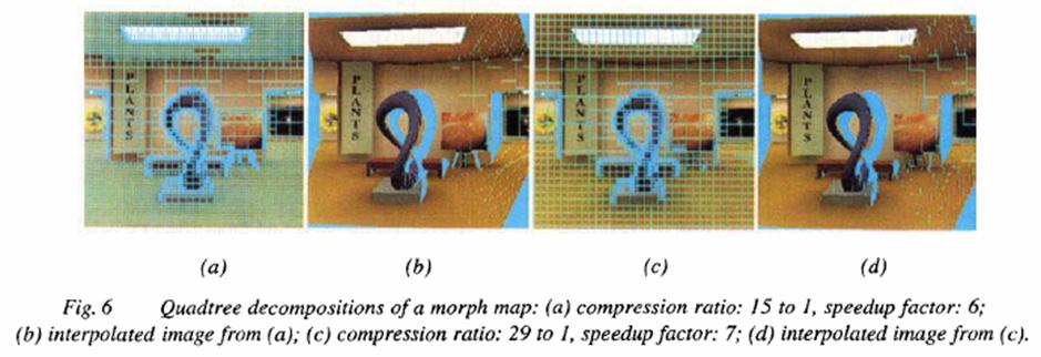
Block Compression
Adjacent pixels tend to move together when being mapped. This allows the use of a block compression algorithm to compress morph map. A block compression has two benefits. The first being the reduction in size of the morph map and the second is that the pixels being blocked together allows groups to be interpolated at once saving processing time. The compression ration of the algorithm depends on the depth complexity of the image. The higher the depth complexity of the scene the lower the compression ratio usually is. The ratio is also lower if the movement of the camera results in a greater pixel depth change. The figure below shows the compression of the image with different max thresholds. Figure a has a max threshold of one pixel and figure c has a max of 2 pixels. What this means is that the offset vectors for adjacent pixels do not differ more that 1 or 2 pixels in a block. The larger of a pixel threshold that you set for the block compression algorithm will cause more pixels to be grouped together and increase the processing speed, but all of this will be at the expense of the image quality.
Applications
There are many applications where the morphing method can be applied. Virtual Reality is one that everyone thinks of right off the bat. The morphing method allows the use of images to perform walkthroughs of environments instead of 3D geometric entities. Every time the view point is change the image in view is interpolated.
Another application where this method could be useful is with motion blur (or temporal anti-aliasing). When an image is sampled from motion at an instance in time but not over a time interval the image will appear jerky and is said to be aliased in the temporal domain. One way to perform anti-aliasing uses super sampling. Samples are taken at a higher rate in the temporal domain and then these samples are filtered to the display rate. This requires a large number of images and becomes computationally expensive thus inefficient. The morphing method would allow additional temporal samples to be created by interpolation at no extra cost to the computation.
The Morphing method could be used to reduce cost of computing a shadow map. Using the shadow buffer algorithm objects can be determined to be in a shadow by their Z value. This algorithm only takes into account point light sources. With multiple light sources you could calculate the shadow map for each light source on the image separately and interpolate them together using the morphing method.
If you’re given images from all different views of an object you would be able to render interpolated views that looked 3D but really were not. As long as we can generate any view of the object it does not matter if the 3D description of the object is actually there.
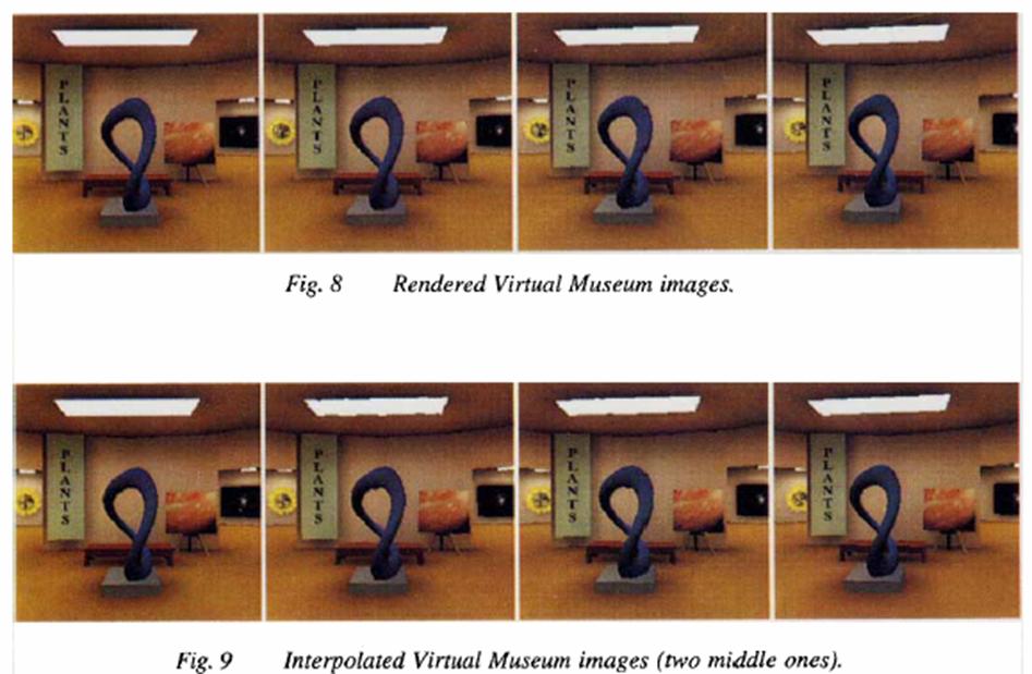
Here are some samples produced using the morphing method.
Plenoptic Modeling
The Plenoptic function is a
function that is able to be used to describe any and all of the image
information that is visible from a specific viewpoint. The Latin root is plenus which means complete
or full and optic meaning
pertaining to vision. It was developed
by Adelson and
“…all the basic visual measurements can be considered to characterize
local change along one or two dimensions of a single function that describes
the structure of the information in the light impinging on an observer.”
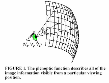
The Plenoptic function in the terms of computer graphics describes the
set of all possible environment maps for a given viewpoint. All that needs to be done to find the view
you’re looking for is to have the correct parameters entered into the
functions.
This includes: (some
of these parameters are shown to the right)
·
viewpoint
(Vx,
Vy, Vz)
·
azimuth
and elevation angle (θ, Ф)
·
in a
dynamic scene we can choose a time t
![]()
Plenoptic Modeling
Plenoptic modeling uses the plenoptic function to generate any viewpoint of a scene. They claimed that all image-based rendering approaches are just attempts to create a plenoptic function with just a sampling of it. Like other models the scene is set up from a set of sampled images. These images are then warped and combined to create representation of the scene from arbitrary viewpoints.
Sample Representation
To be able to use the plenoptic function the have to be able to map they’re sampled images to a geometric model. The most nature surface would be a unit sphere. This would allow an even view from every angel but the problem with this is the storage on a computer is difficult. This difficulty would cause distortions in the image.
The next option discussed was a cube with six planar projections. This would allow for easy storage on a computer but the 90 degree face would require an expensive lens system to avoid distortion. Also the corners would cause over-sampling.
The option the chose is the cylinder. The can be easily unrolled producing a simple planar surface for storage. I also allows for and expansive range to be covered from viewing. The only problem that comes with the cylinder is the finite height which would cause problems with the boundary conditions. To solve this problem they just took off the end caps.
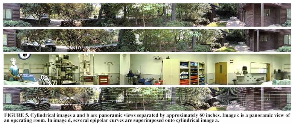
Acquiring Cylindrical Projections
Now that they have the shape of the model they need to gather the sample projections. Getting the projections is actually pretty simple. All that is needed is a tripod that can continuously pan and record all the surroundings. Ideally the camera’s panning motion should be at the exact center of tripod to prevent any of the images from being distorted. When panning objects that are far away a slight misalignment is tolerated. The panning takes place entirely on the x-z plane and both images should have points within each other to allow for the combining of the images later. The projection of the output camera on input cameras image plane is found. This is the intersection of the line joining the two camera locations with the input camera’s image plane. The line joining the two cameras is the epipolar line. The intersection with the image plane is the epipolar point. Now all that’s left is to map the image points to output cylinder. The images below show some of the panoramic views obtained with the camera.
References
§[1] Chen S E and Williams L, "View Interpolation for Image Synthesis", Proc. ACM SIGGRAPH '93 McMillan L, and Bishop, "Plenoptic Modeling: An Image-based Rendering System", Proc. ACM SIGGRAPH '95
§[2] Shade, Gortler, He and Szeliski, "Layered-Depth Images", Proc. ACM SIGGRAPH '98
§[3] McMillan L. and Gortler S,"Applications of Computer Vision to Computer Graphics: Image-Based Rendering - A New Interface Between Computer Vision and Computer Graphics, ACM SIGGRAPH Computer Graphics Newsletter, vol 33, No. 4, November 1999
§[4] Shum, Heung-Yeung and Kang, Sing Bing, A Review of Image-based Rendering Techniques, Microsoft Research
§[5] Watt, 3D Graphics 2000, Image-based rendering and phto-modeling (Ch 16)
§http://www.widearea.co.uk/designer/anti.html
§http://www.dai.ed.ac.uk/CVonline/LOCAL_COPIES/EPSRC_SSAZ/node18.html
§http://www.cs.northwestern.edu/~watsonb/school/teaching/395.2/presentations/14