Look at a N-point median filter. The basic operation is to sort values in rank from 0 to N-1 or 1 to N.
Begin by sorting the values in ascending order. If N is odd, select the middle value, (N+1)/2. If your index originally ran from 0 to N-1, select the N/2 member. This is the median value. If N is even, the result is ambiguous since there is no median value.
In median filtering in image processing, filter spans of 3x3, 5x5, 9x9, etc. are used. The number of pixel values to sort can become large. What is the inherent computational complexity of this operation?
Sorting N items has inherent computational complexity![]() . Sorting
the items in an NxN median filter span has complexity
. Sorting
the items in an NxN median filter span has complexity
![]()
If the image being median filtered is MxM pixels, the complexity becomes
![]()
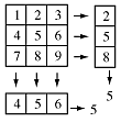
How can this be reduced? One traditional method used to reduce the complexity of 2D operations is to separte them into 1D operations. For example, we could find the median of each column to get a row vector of medians and take the median of that vector. Or, we could find the median of each row to get a column vector of medians and take the median of that vector. Unfortunately, the median filter is not generally separable; those two methods can give different answers and both may be different from the (correct) 2D median. Here is an example which gives the correct result when the medians are calculated separately
And here is one in which the results are different (but one is correct):
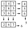
In Homework 3 you are asked to find an example of a 3x3 matrix in which the row-first, column-first, and correct values are all distinct. Hint: it can be done using only the values 1-9.
Consider a pipeline architecture in which each value has an associated rank. Begin by entering the values 2, 7, 5, 3, 1 into the pipeline and then add in a 0, which displaces the 1:
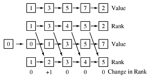
The rank moves along with the old value except that it can change depending on where the new value added to the pipeline fits in. Specifically, the rank associated with a value changes only when the value is between the discard value (the 2 in this case) and the new value (0 in this case). The change is either zero or +/- one:

Thus we know how to update the rank of existing values. How about the rank of the new value? Note that the sum of the ranks is a constant:
![]()
Thus the rank of the new value can be computed by subtracting the sum of the changes in the ranks of the remaining values from the discarded value's rank:
![]()
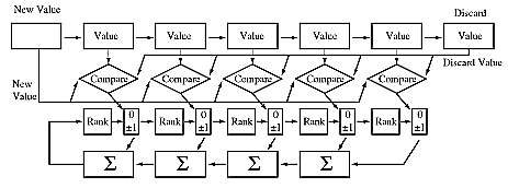
Here is a schematic drawing of a cellular pipeline architecture which implements this algorithm:
Median Filters:
Derivative Operators
Edge Detectors
Gaussians, their transforms and approximation of other operators using differences of Gaussians.
It is difficult to model an imaging system using differential equations, which is unfortunate since a large class of differential equations can actually be solved. Many of the interesting properties of imaging sytems can be modeled using integral equations, but they have a nasty property: almost none can be solved. By using linear system theory we reach a compromise between accuracy and utility of the model versus ability to solve the model. And it is a classical compromise - the dissatisfaction is equally distributed to all participants.
The Fourier transforms of a function is an integral of the form
![]()
and its inverse function is
![]()
The exponential kernel is what makes it a Fourier transform -
other integral transformations have other kernels. Two subjects of great
religious debate among applied mathematician is where, precisely, to put
the ![]() and whether to use i or j to represent
and whether to use i or j to represent ![]() .
.
In practice, these integrals are never actually evaluated, although we did evaluate one instance in class to show why they are never evaluated in practice. Tables of transforms for the few classes of functions which have exact, symbolic solutions are used instead. Also, tables of properties are used to show how manipulations of the transforms F(u) correspond to manipulations of the complementary function f(x). In particular, convolution - an integral that is generally difficult to evaluate - becomes a product of transforms:
![]()
We showed how point spread functions or impulses responses,
such as ![]() are used to characterize imaging systems. In particular, we looked at
the sampling function
are used to characterize imaging systems. In particular, we looked at
the sampling function
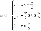

and we derived its Fourier transform:
![]()
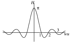
The zero crossings are at integral values of wu, which are seen to be inherently bound together. Thus, as w becomes smaller (smaller pixel size), the central peak of H widens, showing that the pixel samples all spatial frequencies about the same. As w becomes larger (larger pixel), the central peak becomes narrower and sharper, showing that the sensitivity falls off quickly as the spatial frequency increases. The pixel size sets the upper bound on spatial frequency. If objects of too high a frequency are imaged, for a given pixel size (frequencies past the first zero crossing), aliasing or moire effects occur, as we demonstrated in class. The tradeoff between sampling size and cutoff frequency, symbolized by the size/frequency pair wu, is sometimes called the uncertainty effect because of its parallel with the Heisenberg uncertainty phenomenon in quantum physics.
Looking at Fourier transforms and obtaining quantative understanding of what they mean is in important skill in image processing.