by Chris Byrd
The work Perlin did in procedural texture generation [2] formed the basis for the work he did in [1]. I will first give an overview of some of the concepts for procedural texture generation. Then I will talk about hypertexture itself, and lastly I will briefly intruduce the ray casting methods used to render hypertexture.
Procedural texture mapping and procedural modeling is the use of a function or set of functions applied to a set of points in order to generate a texture. One of the most well known methods of procedural texture mapping is probally the use of fractal techniques to generate terrain. There are two main reasons for wanting to use this method to generate textures. One is that because of the use of function to define the texture it is easy to introduce time-varying variable to your model thus creating animation. The other benefit is to be able to specify a highly complex texture with minimal amounts of data storage.
There are a couple additional benefits of a procedural approach to generating textures when you move into three dimensions. One of the other possibilities for getting texture onto a three dimensional object is to map a 2D texture onto the 3D object surface. This might work well with simple objects, however once you get 3D objects that exhibit any great amount of complexity useing the 2D mapping technique can become problematic. With procedural mapping all you need to know is a points location in space. Using that location you can determine what the value of the texture field at that point. This method has been called 'solid textureing'. The only limitation to this method is that you need to be able to define the texture by a set of functions. So mapping a picture taken from a digital camera would not be possible using this method.
One of the common solid texturing techniques is to use a noise function to simulate turbulence. Perlin[2] developed some turbulence models for solid texturing and he extended them to also work with hypertexture. A more in depth talk about noise generation was given by Prof. Ward here . The basic idea is to define a 3D array(lattice) of random numbers. The amount of noise applied to any spot is the random value located at the corresponding location in the array. If the location in space does not correspond with an exact location in the array, various different interpolation methods can be applied to approximate the value using neighboring values in the lattice. Turbulence is defined as summation of noise useing the following equation:
Using this model many realistic textures, such as those of marble or flames can be created.
Hypertexture is an extension of the solid textures. One of the main distinctions between sold textures and hypertexture is that hypertexture objects have no well defined boundaries. Instead thay have a density function that describes how the object should behave in the area where it transitions between the outside and inside of the object.
An object in Hypertexture is partitioned into three different regions. A hard region, a soft region and an outside region. The hard region represents a part of the object where it is completely solid. The soft region represents a part of the object where the density is variable, and the outside region represents where the object is non-existant. The essence of hypertexture is the definition of functions that modify the behavior of the density of an object within its soft region.
There are two main functions that define a hypertexture.
Those are the Object Density Function, D(x), and the Density
Modulation Function (DMF), f.
The Density function, D(x),
describes the density of the object for all points thoughout R^3.
D(x) has a range of of 0 to 1. A value of 1 means the object is
completely solid at that point. A value of 0 means the object has no
density at that point. All values of D(x) such that 0 < D(x) < 1,
represent the objects soft region.
The Density Modulation Function are the functions that control the
behavior of the density within an objects soft region. Perlin
defines a set of base DMF's that can be used as building blocks to
define any hypertexture you want, the functions he defines will be
discussed shortly. A DMF is applied to an objects density function.
Multiple DMF's can be applied to the same D(x).
Hypertexture is formally defined as:
H(D(x),x)= fn(...f2(f1(f0(D(x)))))
Where f0, f1, ... fn are all DMF's.
D(x) =
	r1 = inner_radius^2 = (r - s/2)^2
	r2 = outer_radius^2 = (r + s/2)^2
	rx = distance_from_center = (x.x - c.x)^2 + (x.y - c.y)^2 + (x.z - c.z)^2
	if(rx<=r1) then 1.0
	else if(rx>=r2) then 0.0
	else (r1-rx)/(r2-r1) /* replace this with whatever you want the density to look like*/
Density modulation functions are used to shape the behavior of an objects density inside of its soft region. The DMF that will be described here are the bias, gain, noise and turbulence functions
 A Bias of 0.25
 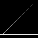 A Bias of 0.7
  A Bias of 0.75
  A gain of 0.25
  A gain of 0.7
 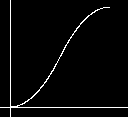 A gain of 0.75
  f1(x)= gain(.25,bias(j,i))
 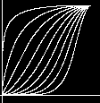 f2(x)= gain(.75,bias(j,i)
(1) Generate a random vector within the interval [-1,1]
(2) if |v| > 1 then goto 1
(3) Normalize the length of v
Turbulence is defined same was as it was in soldid texturing, a summation
of noise:
Hypertexture is rendered using volume rendering techniques. This is the easiest method because hypertexture objects do not always have well defined surfaces.
A ray marching algorithm is used to render hypertexture images.
A ray is cast into each pixel in space, on each ray it is
tested wether or not that ray intersects the parallelpiped that
bounds the hypertexture object. If the ray does intersect with
the bounding volume then its entry and exit points are calculated.
We begin at the entry point and and 'march' down the ray in
some increment, sampling values along the way. We keep doing this
till we hit the exit point of the parallelpiped.
The points along the ray that we stop along are defined as follows:
x = x_0 + K * delta_u
Along each sampleing point of the ray, we calculate the DMF, f(x) at that location. If 0 < f(x) < 1 then the gradient at that point is estimated and then used to calculate the normal vector for that point. The normal vector can in turn be used to calculate things like shading, reflection etc.
To compute the gradient we need 3 points that are perpendicular
to each other. The first point can be f(x-delta_u) since that
is already computed. The other two vectors delta_v and delta_w
are any other two vectors that are all mutually perpendicular.
We put these together to give us the vector:
gradient_f = [ f(x) - f(x-delta_u), f(x+delta_v)-f(x), f(x+delta_w)+f(x) ]
This resulting vector is in (u,v,w) space, to convert it to (x,y,z) space
it is multiplied by the following matrix:
| delta_x  |
| delta_v  |
| delta_w  |
	t = o_k (1-o)
	color = color + t*color_k
	o_k = o + t
 Turbulent sphere
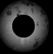 Same sphere, different bias
 Noisy sphere
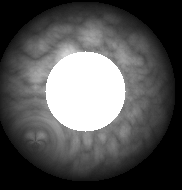
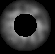 Another Noisy sphere
[1] Perlin, K Hypertexture, Computer Graphics 1989, 253-62
[2] Perlin, K. An Image Synthesizer. Computer Graphics 1985, 287-296
[3]http://www.mrl.nyu.edu/hyper/hypertexture/hypertexture.ps
[4] Alan Watt, Mark Watt. Advanced Animation and Rendering Techniques